
Days of Cover Can Lie When Demand Is Seasonal
A healthy stock total can hide a shortage before the next delivery. Build a dated coverage path that separates commitments, promotional demand, usable receipts and unserved orders.

7 years of experience building and operating brand websites, specializing in website development, paid advertising and SEO. Built a brand website from launch to US$10 million in annual sales.
The Short Answer
Use days of cover as a screening ratio, then check a dated supply-demand path. Reconcile the sellable stock pool, count commitments once, place receipts when they become usable and record what happens to unmet demand. A positive ending balance does not prove that every earlier requirement was served.
Key takeaways
- Gross on-hand units can include stock already committed or unavailable.
- A future average still hides the order in which demand arrives.
- A receipt after the first short date cannot repair earlier service.
- Lost sales can leave more ending stock than delayed fulfillment.
- Forecast consumption and stock reservations must not deduct the same obligation twice.
- The last feasible action date belongs beside the first shortage date.

The inventory dashboard says a product has three weeks of stock. The marketing calendar says a promotion starts on Friday. The next purchase order arrives after the promotion. All three statements can be correct, and the business can still run out halfway through the event.
Days of cover is a useful shorthand only when its numerator, demand rate and time assumptions fit the decision. Dividing a stock total by average daily sales removes the sequence of events. That sequence is often the most important part of the problem: what is available now, what is already committed, when demand changes, and when replenishment becomes usable.
I would use a simple coverage ratio as a screening signal, then use a dated inventory path for any meaningful buying or promotion decision. The path does not need to be complicated. It needs to preserve the timing that the ratio hides. A clear fourteen-day schedule can be more useful than a sophisticated score built from mixed stock states.
This guide works through a fictional brand, Aster Garden, and one product sold during a planned promotion. Every quantity, date index and outcome is illustrative. The examples are calculations for stated scenarios, not measured client results or a claim that a forecast can guarantee availability.
First, say which kind of coverage you mean
Operational days of cover usually asks how long a quantity of stock can support a specified demand rate or future demand schedule. Financial days of inventory uses an inventory value and cost-of-sales relationship over a period. The two measures can share similar names while answering different questions.
A buyer deciding whether a specific warehouse can support next week’s promotion needs units, timing and location. A finance team assessing working capital may need average inventory at cost and cost of goods sold. Substituting one measure for the other can produce a polished number with little relevance to the decision.
Even within operational planning, several coverage measures are possible. Gross on-hand coverage includes everything physically recorded. Sellable coverage excludes unusable stock. Uncommitted coverage also considers existing allocations. Forward coverage compares stock against expected future demand rather than a historical average. Each can be legitimate when labeled and used appropriately.
Write the definition in a sentence beside the number. For example, uncommitted sellable units in the east warehouse divided by the last twenty-eight complete available selling days’ average demand. That is far more interpretable than twenty-one days. It also exposes whether the denominator is sales, eligible orders, shipments or an adjusted estimate of demand.
Do not make the label carry more certainty than the inputs. If warehouse stock is stale, demand history is incomplete or future promotion demand is a scenario, say so. A decimal such as sixteen point four days does not become accurate because the calculation is precise.
The earlier guide on building the right demand history explains why orders, fulfillment and refunds should remain distinct. Coverage inherits that decision. If the demand basis is inconsistent, the resulting depletion estimate will also be inconsistent.
Build a stock waterfall before dividing anything
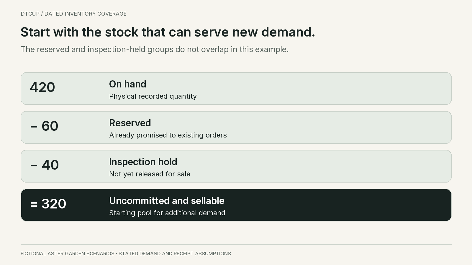
Aster Garden’s fictional stock record shows four hundred and twenty units on hand. Sixty are reserved for accepted customer orders. Forty are in a separate inspection hold and cannot yet be sold. These groups do not overlap. The uncommitted sellable quantity for new demand is therefore three hundred and twenty units.
At a historical rate of twenty units per day, gross on-hand coverage is twenty-one days. Uncommitted sellable coverage is sixteen days. The first ratio counts stock that cannot serve the new demand being considered. Neither ratio yet reflects the approaching promotion.
The arithmetic is simple, but the definitions require care. In another system, available stock might already exclude reservations or holds. Subtracting those quantities again would understate supply. Do not infer the meaning of a field from its label alone; trace the source definition and reconcile a sample item.
Keep the stock snapshot and its timestamp. A purchase order created at noon should not be combined casually with an on-hand balance from last week. If different sources update at different intervals, make the mismatch visible and assess whether it changes the decision. The right response to stale data may be a stock check rather than a new forecast model.
Also distinguish a reservation from physical removal. Reserved units may still be in the warehouse. They are committed to an existing obligation, not newly available for a promotion. If the planning schedule includes those existing orders as future demand, start from sellable stock before reservations and subtract them on their requirement dates. If starting from uncommitted stock after reservations, do not subtract the same commitments again.
For the main Aster example, we start with three hundred and twenty uncommitted sellable units and model only additional demand. The sixty reserved units and forty held units remain outside this new-demand pool. This explicit boundary keeps the later schedule from double-counting obligations or treating held goods as usable.
Replace a flat average with the demand expected on each date
The next fourteen days are not expected to resemble the recent average. Aster plans four ordinary days at twenty units per day, followed by six promotion days at fifty units per day, then four ordinary days at twenty. Total scenario demand is four hundred and sixty units.
The average over those fourteen future days is about thirty-two point nine units. Dividing three hundred and twenty by that average gives roughly nine point seven days. This is closer to the coming demand level than the historical sixteen-day figure, but it still loses the sequence. Demand is not evenly distributed across the period.
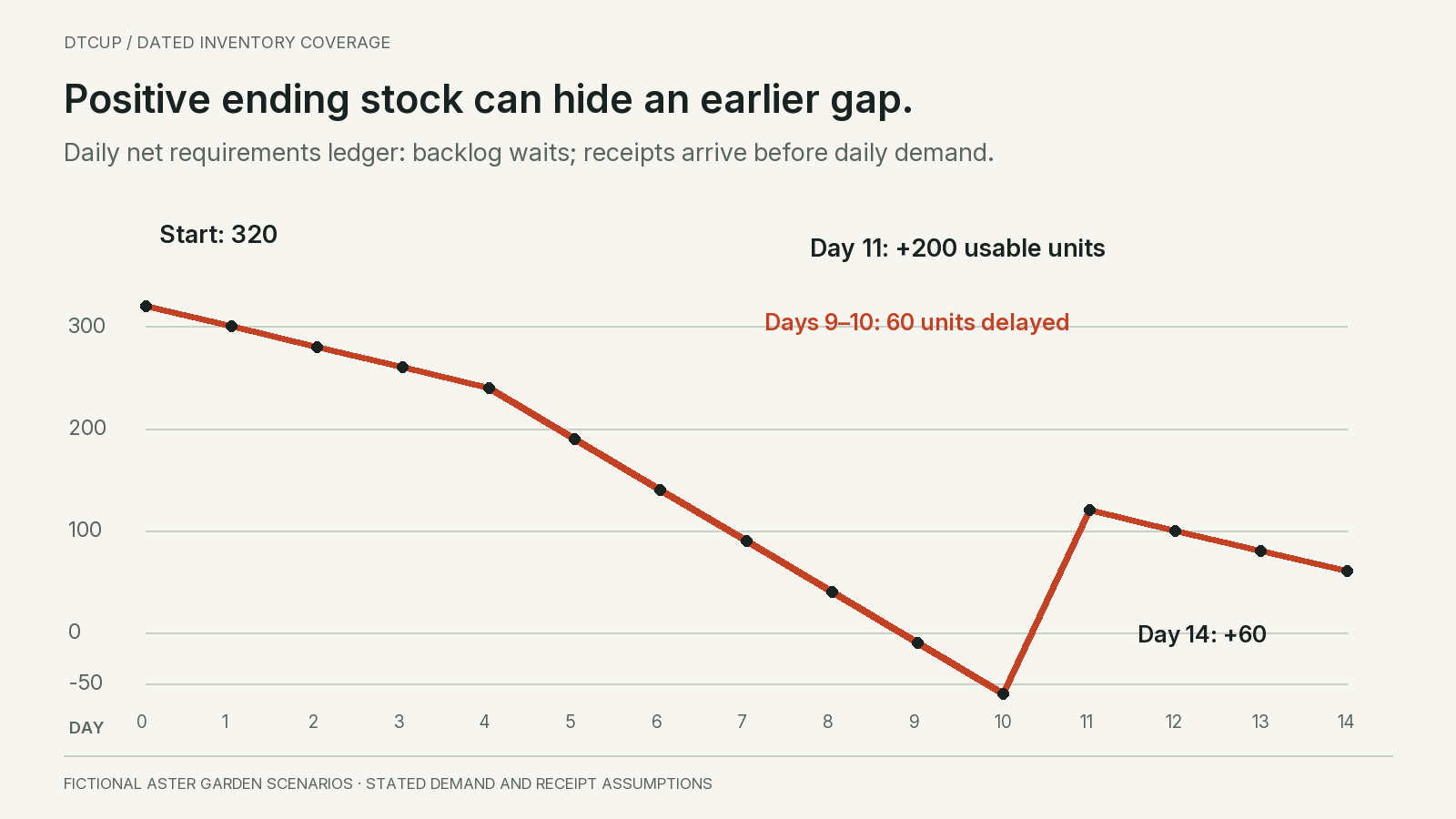
After the first four days, eighty units have been used and two hundred and forty remain. Four promotion days consume two hundred more, leaving forty at the end of day eight. Day nine requires fifty. Under the scenario, the available pool becomes insufficient during day nine.
A simple within-day interpolation would place depletion eight point eight days after the start: eight complete days plus forty divided by fifty of day nine. That fractional value assumes demand is spread evenly within the day. If orders arrive in a morning spike, the actual operational timing could be much earlier. For daily planning, first shortage on day nine is often the more honest label.
The promotion demand is an assumption, not a fact merely because it appears in a calendar. Record its basis: a comparable event, a planned exposure level, a confirmed customer commitment or a scenario chosen for stress testing. Do not add a seasonal multiplier and a promotion uplift if both represent the same expected increase.
A known one-off promotion is also not evidence of stable annual seasonality. New products may have too little history to estimate a repeating seasonal pattern. The plan can still include the event explicitly while keeping uncertainty visible. The article on short-history forecasting develops that distinction.
A future receipt does not repair a past shortage
Aster has two hundred units expected to become usable on the morning of day eleven. Adding those units to the initial three hundred and twenty gives five hundred and twenty units of total planned supply. Total fourteen-day demand is four hundred and sixty. A period-total calculation therefore shows sixty units left over.
That positive ending balance does not mean every day is covered. The receipt arrives after the shortage begins. Forty units remain at the end of day eight, ten units of day-nine demand cannot be served, and fifty units of day-ten demand cannot be served before the new stock arrives.
The timing of usable supply matters more than the date printed on a purchase order. A supplier’s dispatch, a port arrival, a warehouse appointment and release after inspection are different events. The main example assumes the two hundred units are actually available for sale before day-eleven demand occurs. If that assumption is wrong, the gap is larger.
Use a clearly defined event order within each planning bucket. Here, usable receipts arrive at the start of the day and demand is then applied. If the truck arrives after the shipping cutoff, treating it as morning supply can create a false promise. Daily buckets are not precise enough for every operation; important same-day constraints may need a finer schedule.
This is why an aggregate inventory-position measure is useful for some replenishment policies but cannot by itself answer whether every customer requirement can be served on time. Quantity and date must be paired. A late receipt can make the final total healthy while customers experience a two-day gap.
Microsoft’s inventory planning documentation illustrates dated requirements and projected accumulated inventory, and discusses seasonal minimum levels. The general lesson for this worksheet is to evaluate the path through time. The calculations here are independent examples, not a tutorial or feature claim about that product.
State whether unmet demand is lost or carried forward
A negative projected balance is an unmet requirement in a planning ledger, not negative physical inventory. What happens next depends on the business. Customers may wait, cancel, buy a substitute or leave. A coverage calculation should not silently choose one outcome.
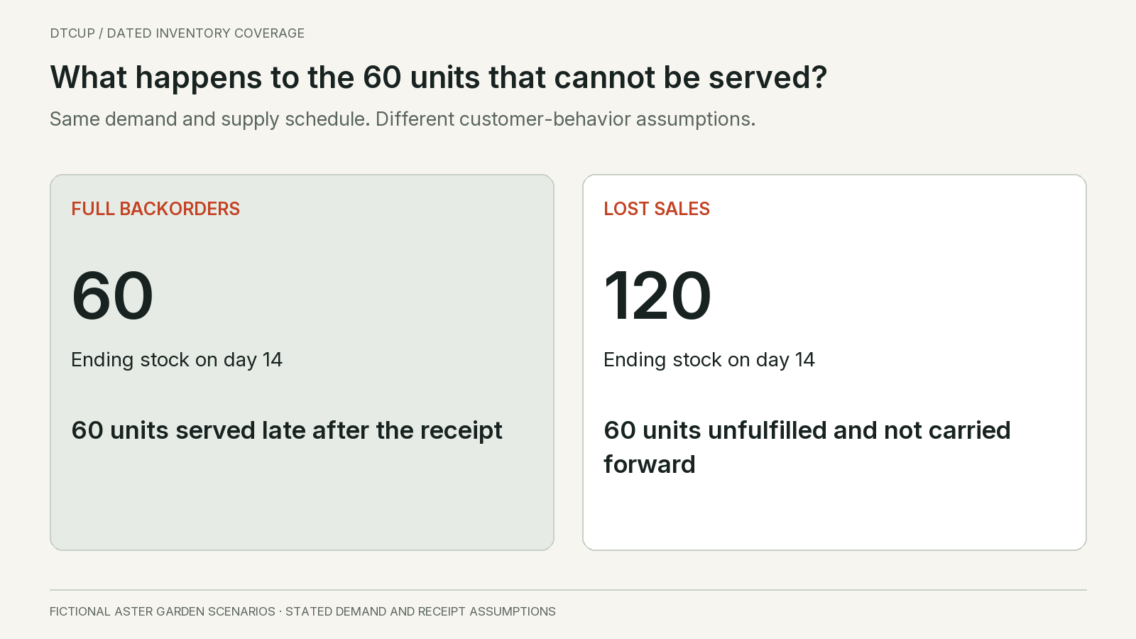
Under a full-backorder version of the Aster scenario, the net requirement balance reaches negative ten at the end of day nine and negative sixty at the end of day ten. The day-eleven receipt adds two hundred, clearing the sixty-unit backlog and supporting twenty units of new demand. The net balance becomes one hundred and twenty, then falls to sixty by day fourteen.
Under a lost-sales version, physical sellable stock stops at zero. Ten units of day-nine demand and fifty of day-ten demand are unfulfilled and do not return. The two hundred-unit day-eleven receipt then serves only new demand. After four ordinary days using eighty units, one hundred and twenty units remain at the end of day fourteen.
The second version ends with more stock precisely because some demand was not served. A dashboard that judges the plan only by ending inventory could mistake that outcome for better coverage. Track unmet demand or delayed service alongside stock, and preserve the assumption about customer behavior.
For mixed behavior, use explicit scenarios. Some customers may accept a delay while others leave. Do not assign a confident percentage without evidence. A bounded range can show whether the action changes under plausible alternatives. The buyer needs to know whether the shortage is a timing inconvenience, a lost-sale risk or both.
Substitution complicates the picture further. Demand lost by one SKU may move to another item, creating pressure elsewhere. Do not count every unfilled request as lost company revenue if customers switch, and do not assume substitution is harmless if it reduces margin or creates another shortage.
The guide to demand hidden by stockouts explains why observed sales can understate demand during these periods. After the event, a zero-sales day should not automatically teach the next forecast that customers wanted nothing.
Prevent accepted orders from being counted twice
Reservations are only one source of double counting. A demand forecast may represent total expected demand, while accepted orders are added separately as if they were entirely extra. The result can inflate requirements and make stock appear less adequate than it is.
Suppose a future day’s total demand forecast is fifty units and thirty units of accepted orders already belong to that forecasted demand. One possible planning convention consumes thirty from the forecast, leaving twenty of residual forecast plus thirty of firm orders. The total requirement remains fifty.
Another day may contain a special wholesale order that was never included in the baseline forecast. In that case, the additional order can genuinely increase the requirement. The system needs a rule for forecast consumption and exceptions; neither always add nor always subtract is safe.
Keep the convention visible in the worksheet. A buyer should know whether forecast demand is total demand or incremental demand beyond existing commitments. That definition must align with the starting stock pool. Subtracting reservations from stock and then adding the same reserved orders to demand creates a second deduction.
Returns can create the opposite mistake. A refund does not automatically create usable inventory. The item may be in transit, damaged, incomplete or waiting for inspection. Count a return as supply only at the appropriate release event and under a justified scenario. Financial reversal and physical recovery are different processes.
Likewise, do not subtract canceled demand twice. If the source order feed already removes canceled quantities from open requirements, an additional cancellation adjustment can understate demand. Reconcile quantities to a few actual source records before trusting a large automated coverage report.
These errors can be larger than the difference between two forecasting methods. I would resolve the stock and demand accounting first. An elaborate seasonal model cannot correct a worksheet that subtracts the same order two times or adds an uninspected return as immediate supply.
Compare changes that actually move the shortage
The dated path gives Aster several concrete options. The buyer might move part of the receipt earlier, the marketing team might reduce the promotion’s demand pressure, or the business might accept a clearly communicated delay. Each option should be modeled as a change to an event, not as an unexplained increase in days of cover.
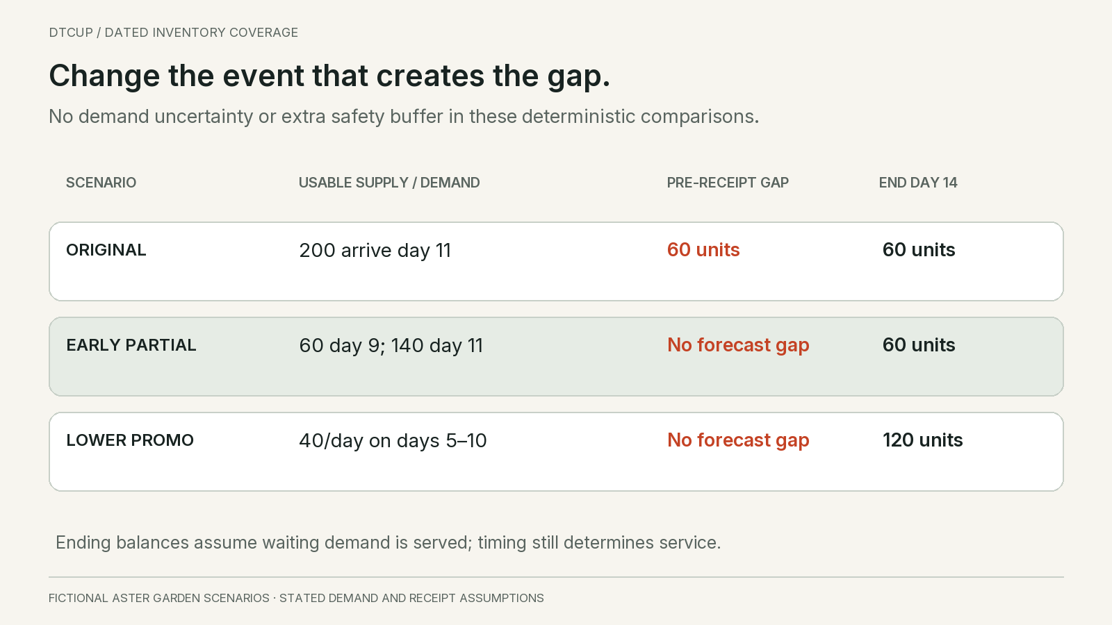
In the main scenario, advancing sixty usable units to the morning of day nine would exactly cover the projected ten-unit gap on day nine and fifty on day ten. The remaining one hundred and forty units could still arrive on day eleven. Under deterministic demand and the stated timing, this removes the shortage and leaves sixty units at day fourteen.
Exactly covering the forecast gap is not the same as providing a buffer. If demand is higher or the early shipment arrives after cutoff, the plan can still fail. The action comparison should therefore show both the expected path and relevant stress cases rather than declaring sixty units a universally safe expedite quantity.
Alternatively, if the entire two hundred-unit receipt arrives on the morning of day nine, the plan has more room through the peak and still ends with sixty units when all four hundred and sixty units of demand are served. That may be operationally easier or more expensive. The decision needs the actual feasibility and cost of each option.
A third scenario reduces promotion demand from fifty to forty units per day for days five through ten. After eighty ordinary units, the six promotion days use two hundred and forty, exactly consuming the initial three hundred and twenty by the end of day ten. The day-eleven receipt then supports the final eighty units, leaving one hundred and twenty.
That scenario is not permission to assume marketing can dial demand to an exact number. It represents an alternative exposure or offer plan whose effect is uncertain. The value is to identify the amount and timing of relief needed, then ask whether a real change can plausibly provide it.
Compare consequences beyond the stock line: expediting cost, missed margin, customer promise, warehouse workload and the risk of excess after the event. A larger order arriving after the promotion may increase ending stock without solving the immediate shortage. The best action is the one that changes the constrained interval at an acceptable cost.
Read coverage differently before and after a peak
A trailing average responds slowly when demand changes direction. Before a seasonal peak, recent low sales can make current stock look abundant. After the peak, recent high sales can make the same stock look scarce and encourage replenishment that arrives too late to be useful.
Consider two products with identical stock and identical trailing thirty-day sales. One is entering its main selling season and the other is leaving it. Their historical coverage ratios are equal. Their future depletion paths and sensible purchasing decisions can be very different.
Use forward demand only when its basis is defensible. Comparable prior seasons can help, but product changes, market expansion, promotions, price and availability can alter the pattern. Preserve those differences rather than copying last year’s curve without explanation.
Check whether last year’s low sales reflected low demand or unavailable stock. A seasonal forecast built from a constrained peak may understate the next peak. Conversely, a one-off bulk order can exaggerate the recurring seasonal pattern. The history needs interpretation before it becomes a future calendar.
For a new seasonal item, show scenarios and decision dates. A first purchase can be staged, a reorder option negotiated, or exposure adjusted as evidence arrives. Do not present a precise annual curve when the business has never observed a complete comparable season.
After the peak, include the remaining selling window and the likely arrival date of any new order. A low current coverage number does not justify a purchase that becomes usable after demand disappears. The buyer may prefer a controlled sellout, substitution or a smaller replenishment depending on the customer promise and economics.
Seasonality changes both expected demand and the value of time. An extra unit available before the event can be useful; the same unit available afterward may tie up cash. A coverage report should help the team see that difference rather than flattening the year into one average rate.
Do not let the total hide the item the customer needs
Company-wide stock can conceal a local shortage. Units in another warehouse may require a transfer, inspection or different shipping cost before they can serve the intended customer. Treat the transfer as a dated receipt at the destination and a corresponding reduction at the source, not as stock that exists in both places.
Variants create a similar problem. A product family may have thirty days of total coverage while its most requested size has three. Customers may not accept another size or color. Aggregate coverage is useful for a portfolio view, but the service decision belongs at the level where substitution is actually possible.
Bundles require component logic. If one kit needs two trays and one clip, abundant trays do not make complete kits available when clips are missing. Convert the intended demand into component requirements, account for other uses of those components, and avoid counting both finished kits and their contained parts as independent supply.
Channel commitments also matter. Stock promised to a wholesale customer may not be available for a website promotion even if both appear in the same warehouse. Reallocating it is a business decision with consequences, not a harmless dashboard adjustment.
Ask the team to define the fulfillment promise before choosing the aggregation level. Can another warehouse meet the deadline? Is substitution accepted? Are units transferable across markets? Are there packaging or compliance differences that make apparently identical goods noninterchangeable? Only verified answers should widen the usable stock pool.
A useful summary can show both the portfolio total and a list of exceptions by item, variant, warehouse and date. That allows leadership to understand the overall position while buyers focus on the constraints that will affect actual orders.
Show uncertainty as alternative paths, not extra decimals
The main Aster schedule assumes fifty units per promotion day and a usable receipt on day eleven. Neither may be certain. A range of plausible demand and receipt scenarios can show whether the proposed action is robust or depends on an optimistic combination.
For example, keep the ordinary days unchanged and consider promotion demand of forty, fifty or sixty units per day. Separately consider receipt availability on day nine, eleven or thirteen. These nine combinations are a stress matrix, not nine equally likely futures unless evidence supports those probabilities.
Look first at the combinations that change the action. If an early partial receipt removes the gap only in the lowest-demand scenario, the plan remains exposed. If a modest timing change protects most plausible paths at a manageable cost, it may be preferable to a large late purchase.
Demand and supply may fail together. A market-wide event can increase orders while suppliers and carriers become busier. Treating high demand and late receipt as independent can understate that joint stress. Include a combined scenario when the business has a credible reason to worry about it.
Keep forecast uncertainty separate from data uncertainty. A wide demand range is one issue; not knowing whether the stock count is current is another. The first may justify a flexible supply response. The second may justify verification. Adding safety stock to compensate for every unknown can hide a broken information process.
When a safety buffer is part of the policy, show the date at which the projected balance falls below it as well as the date of physical shortage. These are different thresholds. The safety-stock guide explains how to connect that buffer to a service decision rather than an arbitrary percentage.
A forecast path is a decision aid, not a promise to the customer. Customer-facing availability should follow the business’s authorized order-promising process, including the relevant commitments and constraints. A planning spreadsheet should not silently become a guarantee of delivery.
Check the calendar edges before trusting the first short date
A daily schedule is only as useful as its calendar. A business may sell every day but receive goods only on weekdays. Its warehouse may accept a Saturday delivery while inspection staff return on Monday. The receipt should enter usable supply when the required process is complete, not when a carrier first reaches the building.
This becomes especially important around holidays. Suppose a supplier says an order will arrive in three business days and the worksheet interprets that as three calendar days. If a weekend sits between dispatch and receipt, the projected stock line can be several days too optimistic. Write the relevant working calendar into the assumption rather than relying on an unexplained lead-time number.
Demand calendars need their own treatment. A shop closed on Sunday can still accept website orders that become Monday requirements. Decide whether the planning date represents order acceptance, picking, shipment or customer need. Moving every Sunday order into Monday may be reasonable for a warehouse workload model but misleading for an order-acceptance promise made on Sunday.
The same discipline applies to time zones and cutoff hours. A purchase order dated Monday in the supplier’s system may not be a Monday morning receipt in the destination warehouse. For ordinary products a conservative daily bucket may be sufficient. For a launch with a narrow fulfillment window, retain the actual local event time and assess whether the goods can pass receiving before the promised shipment.
There is also an important limit at the end of the forecast. If the worksheet contains fourteen days and stock never runs out, the supported conclusion is that the scenario covers the modeled fourteen days. It is not an exact depletion date beyond that horizon. Extend the relevant demand schedule before claiming twenty or thirty days of forward cover.
A zero-demand interval should not produce a reassuring infinity symbol without explanation. Perhaps the product is between seasons, temporarily inactive or missing demand data. Each explanation changes the action. Show no modeled demand within this horizon, with the reason and the next review date, rather than treating division by zero as proof that the inventory is healthy.
Expiry and end-of-sale restrictions create another calendar edge. A lot can be physically present today but become unusable before later demand arrives. If that matters to the product, record the removal or eligibility change on the appropriate date and allocate demand to eligible lots under the business’s actual rule. A single undated quantity cannot represent stock that stops being usable halfway through the plan.
These details do not require every business to build a complex scheduling engine. They require the team to identify which calendar assumptions could reverse its decision. Start with those. Adding minute-level precision everywhere creates maintenance work; ignoring a known weekend inspection closure can create a preventable shortage.
Separate the warning date from the failure date
Aster’s physical shortage begins on day nine in the main scenario, but waiting until day nine to respond would be too late. The supplier may require three days to split a shipment, and the warehouse may need a receiving appointment. The last practical decision date therefore falls before the first short date. Put both dates in the exception.
The warning threshold can also include a service buffer. Suppose, solely as a policy illustration, Aster wants at least sixty units remaining during the promotion. The original path has ninety units at the end of day seven and forty at the end of day eight. It breaches that sixty-unit policy threshold on day eight, then reaches an actual shortage on day nine.
Those sixty buffer units are not an additional physical hold in this example. They are a preferred minimum against uncertainty. Deducting them from stock as if they were unavailable, then also testing the balance against a sixty-unit threshold, would count the protection twice. Keep usable quantity and the desired minimum as separate fields.
A threshold breach should trigger a proportionate review rather than an automatic emergency purchase. Check whether the demand scenario changed, whether a receipt is confirmed and whether the service objective still applies. If the promotion has been canceled, the warning may no longer describe the current plan. If the receipt is delayed, the same warning may now deserve more urgent action.
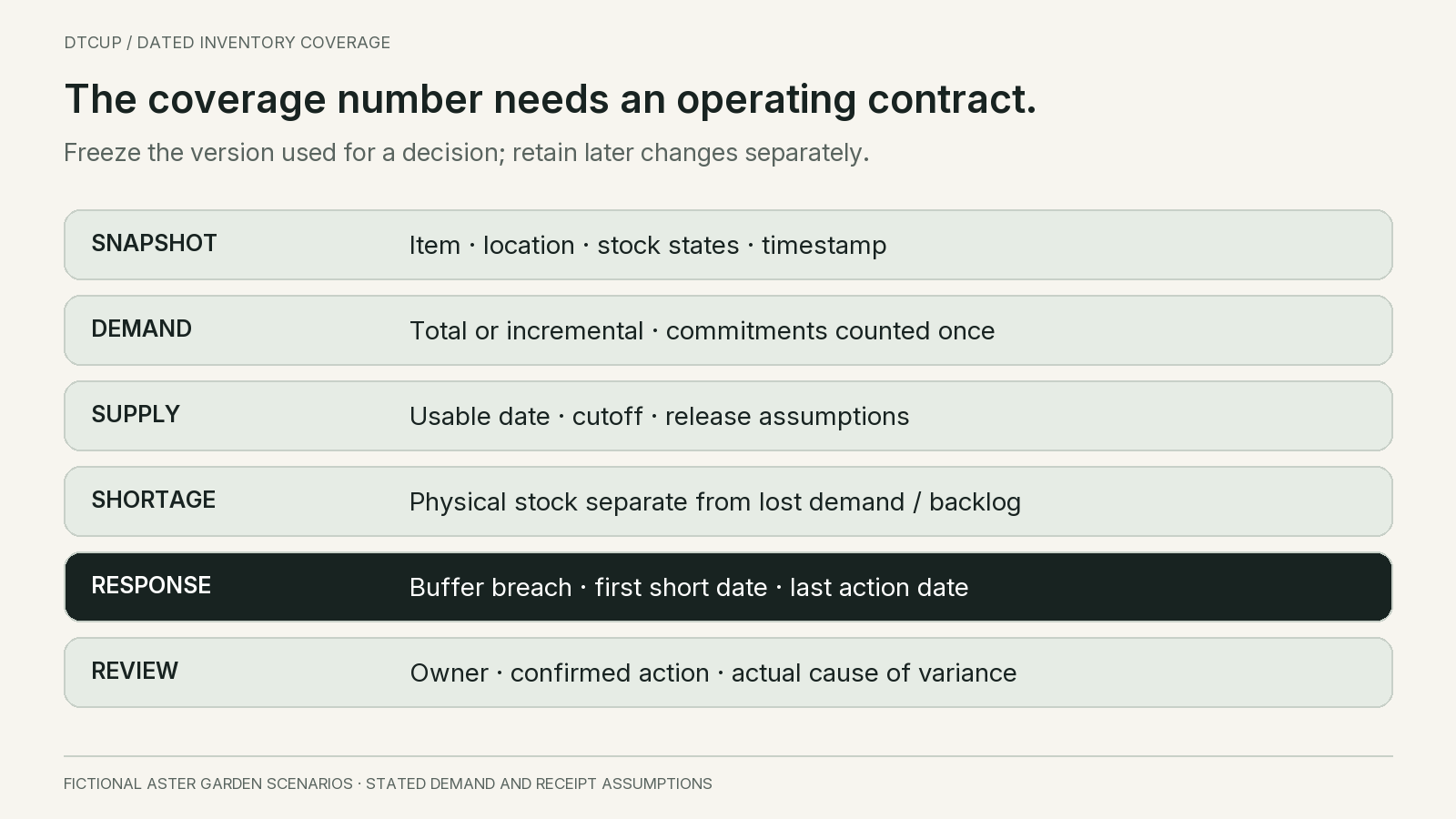
Use a second checkpoint after an action is confirmed. An expedited shipment that merely leaves the supplier does not complete the recovery. Compare its expected usable date with the constrained interval and retain an owner until receipt and release are verified. Otherwise, the dashboard can turn green when the buyer clicks approved even though customers remain exposed.
I would measure the process by actionable notice and explained outcomes, not by how many alerts it produces. An alert issued early enough to change a shipment is useful. Ten repeated alerts with no owner are noise. After the event, record whether the warning was timely, whether the chosen action was feasible and which assumption actually determined service. That feedback improves the operating process around the coverage calculation.
Build the smallest worksheet that preserves the important events
Start with one item and one location. Record the snapshot date and time, the stock-state reconciliation, the demand convention and the scenario name. Then create one row per day across the decision horizon. Use a longer or shorter bucket only when it still preserves the constraints that matter.
Each row needs opening usable stock or net requirement balance, usable receipts, the defined demand requirement, ending balance and any unmet or delayed quantity. Add notes for promotion changes, receipt assumptions and important cutoff times. Keep physical stock and backlog separate if the business can carry unfulfilled orders.
For a backorder ledger, the simple net balance recurrence is previous net balance plus usable receipts minus requirements. Negative values represent outstanding requirements. For a lost-sales ledger, physical ending stock cannot fall below zero; unmet demand is recorded separately. Choose the recurrence deliberately rather than letting spreadsheet formatting decide.
Reconcile the horizon total as a second check, while remembering its limit. Beginning supply plus receipts minus served demand should explain ending physical stock. If demand is lost, it must appear in the unmet ledger rather than disappear from the analysis. If backorders remain, the net requirement record should explain them.
Keep manual overrides visible. A buyer may change a receipt date based on a supplier update or adjust promotion demand after a marketing decision. Record who changed what, why and when. Otherwise, a later review cannot distinguish forecast error from an undocumented change in assumptions.
Save a frozen version at the decision point. Comparing the final actual outcome against a forecast that was repeatedly overwritten during the event produces misleading accuracy. The decision should be evaluated against the information available when it was made, with later updates retained as separate versions.
The method in backtesting the purchase decision extends this idea across historical decision dates. First make one current schedule understandable. Then automate and evaluate the same logic across more items.
Turn the exception into a decision before the deadline passes
A warning that says low cover is not enough. The useful exception states the affected item and location, first short date, quantity at risk, expected usable receipt date, confidence in the inputs and the latest date for a feasible response.
For Aster, the initial exception is specific: new-demand stock becomes insufficient on day nine, with sixty units of demand exposed before a day-eleven receipt under the promotion scenario. An early partial shipment could close that forecast gap if it is usable before day-nine demand. The buyer can now ask a supplier a concrete question.
Marketing needs a similarly concrete request. If earlier supply is not feasible, which exposure or offer change could reduce demand pressure during days nine and ten? Would the business rather accept delayed fulfillment with accurate communication? The answer depends on the customer promise, economics and operational capability, not just the stock ratio.
Assign one owner to each action and keep its state visible: proposed, confirmed, in progress or completed. A supplier discussion is not a confirmed early receipt. An approved transfer is not usable destination inventory. The coverage path should reflect the best supported state, with alternative scenarios where commitments remain uncertain.
Review the result after the event. Did demand differ, did the receipt arrive late, or did the stock snapshot contain an error? These causes lead to different improvements. Raising every future coverage target because one event failed can create excess without fixing the underlying issue.
The operating value comes from acting while options remain. A perfect explanation produced after the promotion cannot recover missed service. Set review timing around the last feasible action date rather than around a convenient monthly reporting cycle.
Questions about days of cover
Is stock divided by average daily sales always wrong?
No. It is a useful descriptive signal when stock and demand definitions are consistent and the rate is relevant. It becomes misleading when treated as a complete future availability plan despite changing demand, commitments, receipt dates or location constraints. Use it to screen, then inspect the dated path for consequential decisions.
Should inbound inventory be included in cover?
It can be included in a dated projection at the point it becomes usable under the stated scenario. Adding all inbound units to today’s stock hides timing and release uncertainty. Keep a current-stock measure and a future supply path separate so that a late receipt cannot conceal an earlier gap.
Why does my model show negative inventory?
A net requirements model can use negative balances to represent demand not yet covered. Physical stock cannot be negative. Label the meaning and specify whether unmet demand waits, is lost or follows another rule. Otherwise, later receipts and ending balances will be interpreted incorrectly.
Can I average coverage across products?
An average may be useful for a clearly defined portfolio summary, but it can hide critical shortages and does not establish substitutability. Show the underlying item and location exceptions. A hundred units of an unwanted variant cannot automatically serve demand for the one that has run out.
What should I check before buying more?
Verify the usable stock pool, demand convention, first short date and feasible arrival date. Then compare a purchase with timing changes, transfers, substitutions and justified changes to exposure. More units arriving after the constrained period may solve the wrong problem and leave the business with unnecessary stock.
Days of cover becomes useful when it leads back to a clear sequence: stock available, demand required, supply arriving and action still possible. Keep that sequence visible. The goal is to protect real customer requirements, not to make a single dashboard number look comfortable.
Sources
Still have a question?Ask the DTCUP Community ↗