
Choose a Demand Forecast by Backtesting the Purchase Decision
A more accurate forecast is not automatically a better purchase. Rehearse six buying cycles, carry inventory forward and test how carton rules, shortages and cost assumptions change the preferred plan.

7 years of experience building and operating brand websites, specializing in website development, paid advertising and SEO. Built a brand website from launch to US$10 million in annual sales.
The Short Answer
Issue historical forecasts using only information available at each decision date, then apply the same executable purchase policy to each method. Carry stock and commitments forward, inspect shortages and remaining inventory, and test uncertain cost assumptions. Separate forecast accuracy from the consequences of the policy built around it.
Key takeaways
- The forecast horizon must match the purchase and replenishment question.
- Historical data and plans must respect each origin’s information cutoff.
- Compare an appropriate simple baseline with the candidate.
- Use the same purchase constraints before attributing differences to the forecast.
- Reconcile inventory sequentially instead of resetting it between cycles.
- Test cost assumptions before turning lower error into a buying recommendation.

A demand forecast can look accurate on a chart and still lead to an expensive purchase. It may predict next week well while missing the period before replenishment arrives. It may reduce average error by overpredicting every product. Or its small improvement may disappear once orders must be rounded to full cartons.
I would choose a forecast by asking two related questions. First, how well would it have predicted demand using only information available at the time? Second, what would the business have bought, stocked and failed to serve if it had used that forecast through its actual planning rules? The first question tests the forecast. The second tests the decision built around it.
This article works through both questions using Bracken Home, a fictional seller of storage pouches. All quantities, predictions and costs are invented teaching data. The example is not a verified saving, an estimate for a real merchant or evidence that one forecasting algorithm is generally superior. Its purpose is to make the comparison reproducible enough that another person can challenge it.
The method is a historical rehearsal. At each decision date, freeze what the buyer could know, generate the forecast, apply a stated purchase policy and compare the resulting plan with later demand. Do not begin by searching for the most sophisticated model. Begin by making the rehearsal honest about time, information, inventory and consequences.
1. Define the purchase decision before choosing an accuracy measure
Write the decision in operational language. Which item or component is being purchased? For which location? When can the purchase become sellable stock? When will the buyer review the item again? What quantity constraints and cash limits apply? A model comparison without these details can optimize a forecast that the purchasing process cannot use.
Suppose a buyer reviews weekly and replenishment normally takes three weeks to become usable. In a periodic review design, the buyer may need to consider demand through the lead time plus the time until the next review’s replenishment can arrive. The precise protection period depends on the policy. A one-week prediction alone does not answer that longer purchase question.
Keep the forecast horizon and ordering policy separate. The forecast describes expected demand over specified future periods. The policy decides how that expectation, uncertainty, usable inventory, inbound stock and constraints translate into a quantity. Adding safety stock does not make the demand forecast more accurate; it changes the inventory decision around uncertainty.
Also distinguish total demand from the weekly path. Two forecasts can both predict 120 units over four weeks while placing demand in different weeks. If stock arrives halfway through, that timing difference can determine whether customers face a shortage. An aggregate horizon total is adequate only when the decision and stock timing make that aggregation acceptable.
Choose the comparison unit accordingly. A purchase made for a particular variant and warehouse cannot be evaluated solely through a brand-wide revenue forecast. A bundle may require component demand rather than finished-kit counts. A transfer between locations needs the destination timing as well as the total business stock.
Before calculating any score, write the loss you are trying to avoid. That may include unserved units, delayed orders, expediting, capital tied up, handling or obsolete stock. Some consequences are measurable directly and others need scenarios. Keep uncertain monetary assumptions visible instead of treating a convenient penalty number as established accounting cost.
For a broader explanation of purchase commitments, usable stock and ownership, see the existing inventory planning guide. Here the narrower objective is to compare forecast methods through a historical decision process, not to redesign every part of purchasing.
2. Reconstruct what was knowable at each decision date
A backtest becomes misleading when it gives the historical buyer information from the future. This can happen without anybody deliberately cheating. Today’s product file contains a corrected category. Today’s order export includes late-arriving orders. Today’s promotion calendar includes campaigns that had not been approved when the purchase was placed.
Define an information cutoff for each origin, meaning the date and time from which the forecast is issued. Only observations and plans available by that cutoff belong in the inputs. A promotion approved two weeks later cannot be used as though the buyer already knew it. A supplier delay discovered after the order should not silently become a known lead-time input.
Where possible, use historical snapshots of stock, open commitments, product status and forecast inputs. If those snapshots do not exist, label the reconstruction. An analysis using today’s cleaned demand history can still compare forecasting behavior, but it cannot fully reproduce what the business would have decided with its original data quality.
Keep revised targets separate from original inputs. It may be appropriate to evaluate against a later, more complete record of eligible demand while training on what was available at the origin. Record both versions. Otherwise a reporting correction may appear to be an impossible prediction error, or the correction may leak backward into the training data.
Check the demand definition before building the timeline. Ordered units, shipped units and refunded units answer different questions. A delayed shipment should not move customer demand into a later week merely because fulfillment happened then. The demand-history reconstruction guide explains the event distinctions that need to be settled first.
Unavailable stock creates another complication: observed orders may understate what customers would have wanted. A method that predicts those suppressed orders accurately can still underbuy. Label constrained periods and decide whether to exclude them for a specific comparison, use a documented estimate or present alternative demand scenarios. Do not pretend an imputed number is an observed fact.
Finally, record missing coverage. If the export begins after the product launch or omits a sales channel, the model is seeing an incomplete business. No amount of historical scoring repairs that absence automatically. Narrow the claim to the observed scope and keep the missing information in the decision notes.
Derived inputs need the same discipline as raw orders. A moving average must end at the origin, not include the week being predicted. A product’s “best seller” label should not be calculated from the full evaluation period and fed into earlier forecasts. A missing-value replacement should not borrow later observations without being labeled as a retrospective reconstruction.
A useful leakage check is to truncate the source at one historical origin and regenerate its inputs from scratch. Compare those inputs with the ones used in the large backtest. If they differ because the large run consulted future rows, the forecast comparison is contaminated. This check is particularly valuable when spreadsheet formulas, feature tables or imported planning files are maintained separately.
3. Move the forecast origin forward instead of mixing past and future
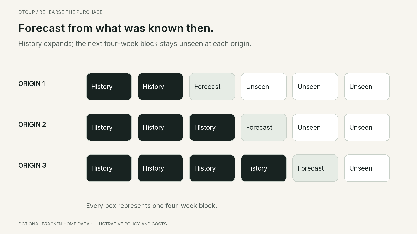
At the first eligible decision date, use the history available up to that date to forecast the required horizon. Save the prediction before revealing the later outcome. Then advance to the next decision date, extend or update the training data as specified, and repeat. Each origin represents another rehearsal of the buyer’s information position.
The forecasting textbook Forecasting: Principles and Practice describes this as evaluation on a rolling forecasting origin. Training observations precede the test observation, and the approach can evaluate multi-step horizons. The Bracken purchase simulation below adds an original operating example; it is not a result from the textbook.
A random split of rows is usually inappropriate for this chronological decision. It can allow later demand patterns to inform an earlier forecast, making the method appear better than it would have been in operation. Keep time order intact, including the sequence used to calculate derived features, choose parameters and approve manual overrides.
Choose origin spacing to match the use case. Weekly purchasing reviews can justify weekly origins. Monthly contract commitments may require a different cadence. Overlapping forecast horizons provide useful observations, but they share many of the same demand periods. Do not count those overlapping observations as independent evidence of repeated business success.
Specify whether the model is refitted at every origin or used unchanged for a period. A method trained once and another retrained weekly are different operating configurations. Either can be reasonable, but the comparison should reflect how each would actually be maintained rather than granting one free access to more current information.
Reserve a later block for a final check after choosing settings. If every historical period is used repeatedly to select model variants and policy parameters, the winning score partly reflects adaptation to that history. A final untouched period will not eliminate uncertainty, but it can expose a method that only fits the development comparison.
Keep the forecast files themselves, not just the summary score. Each saved record should identify origin, target period, item, location, method and predicted quantity. This allows the buyer to inspect whether the apparent gain comes from one extraordinary period, a systematic bias or a repeatable improvement across several decisions.
4. Give a simple baseline a fair comparison
A candidate forecast needs a reference point. For a stable item, a recent average or last-period value may be a useful baseline. For a genuinely seasonal item with sufficient comparable history, a seasonal reference may be more appropriate. The baseline should fit the decision and available evidence, not be deliberately weak so that a complex method can defeat it.
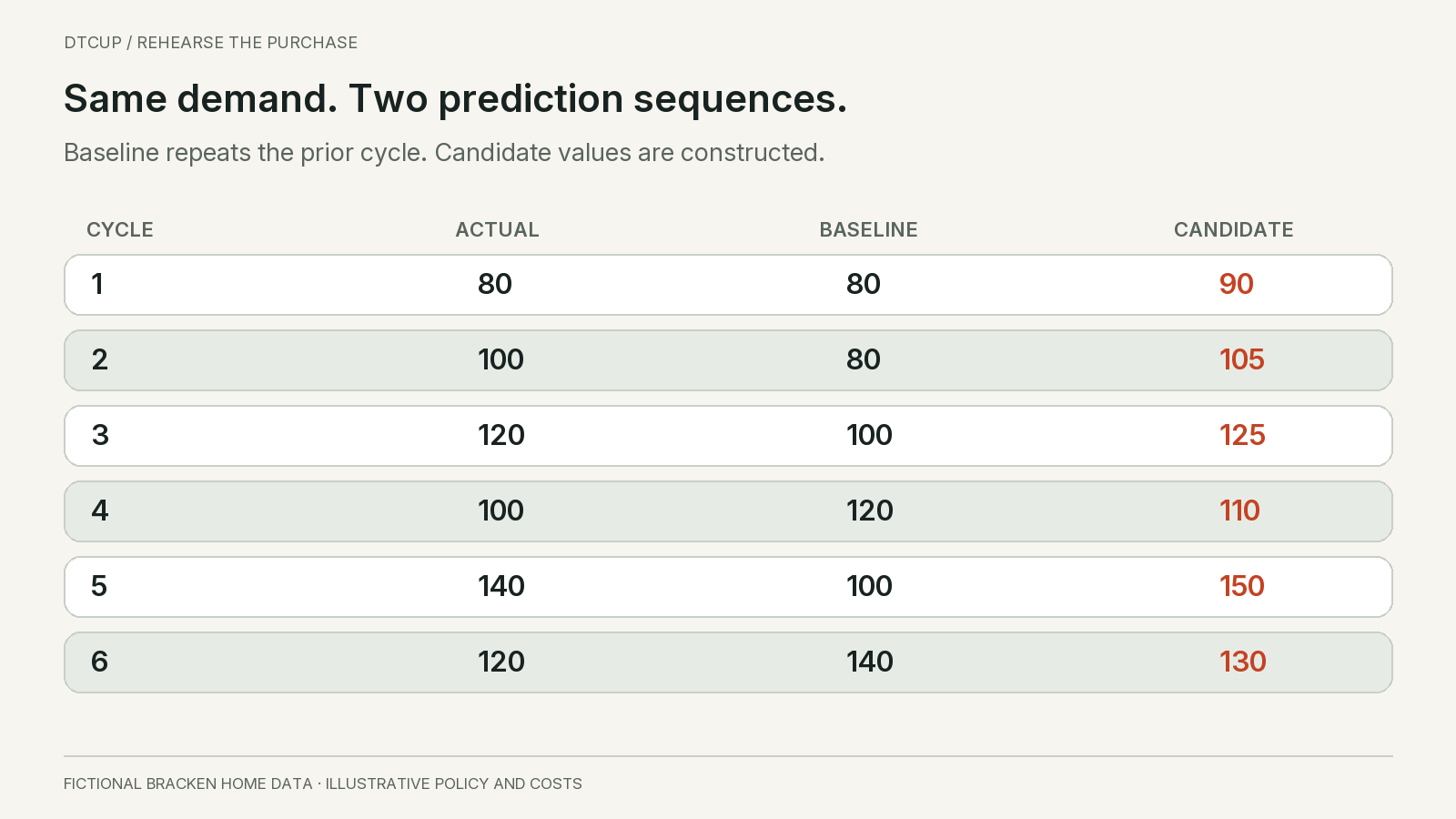
Bracken’s teaching case uses consecutive four-week cycles. The complete, unconstrained demand in the cycle before evaluation is 80 units. Demand in the six evaluated cycles is 80, 100, 120, 100, 140 and 120 units. Each cycle’s total becomes known only after that cycle closes.
The baseline predicts that the next four-week cycle will match the previous cycle. Its forecasts are therefore 80, 80, 100, 120, 100 and 140 units. This is a deliberately transparent rule, so every prediction can be traced to information available before the next cycle begins. It is not a claim that last-cycle demand is suitable for every product.
The candidate’s saved predictions are 90, 105, 125, 110, 150 and 130 units. These numbers are constructed to illustrate comparison; they are not outputs of a trained model or evidence that a particular algorithm can achieve them. In real work, each would need a dated forecast file generated by the candidate using the permitted historical inputs.
Both methods forecast the same item, unit, location and target cycle. Neither gets advance knowledge of the realized demand. For the arithmetic example, demand is assumed fully observed and unaffected by availability. That assumption makes the comparison readable; real stockout-censored history requires the separate treatment described in the stockout-demand guide.
Do not compare a candidate’s four-week total with a baseline’s one-week error and call the result an improvement. Likewise, do not give one method a manually corrected promotion forecast while leaving the other on raw history unless the intended comparison explicitly includes that human intervention.
A useful baseline also acts as a diagnostic. If a complicated method repeatedly loses to a simple reference, investigate whether the additional inputs are noisy, unavailable at the origin or describing the wrong demand. Complexity can still be worthwhile for a different horizon or product class, but the burden of proof belongs to the actual decision.
5. Inspect error direction and distribution before buying anything
Use an explicit sign convention. Here forecast error means predicted demand minus actual demand. Positive error means overprediction; negative error means underprediction. Another report may use the reverse convention, so write the definition beside the calculation rather than assuming the word “bias” has a universal sign.
The baseline’s six errors are zero, minus 20, minus 20, plus 20, minus 40 and plus 20 units. Its absolute errors sum to 120 units, giving mean absolute error of 20 units per four-week cycle. Its signed errors sum to minus 40, which signals net underprediction across this small example.
The candidate’s errors are plus 10, plus 5, plus 5, plus 10, plus 10 and plus 10 units. Absolute error totals 50, giving mean absolute error of about 8.33 units. Its signed total is plus 50. It is closer on average, but it overpredicts in every evaluated cycle.
Neither observation should be hidden. The candidate improves this symmetric error measure. It also has a persistent directional tendency. Whether that tendency produces an acceptable purchase depends on the policy, demand uncertainty, stock constraints and consequences of surplus. “Lower error” is a factual description of this metric, not yet a purchasing recommendation.
Look at the worst relevant miss as well as the average. The baseline misses cycle five by 40 units, while the candidate exceeds it by 10. If cycle five contains a high-consequence promise or a product that cannot be replenished quickly, that difference may matter more than several small improvements elsewhere.
Do not cancel positive and negative errors and call the result accurate. A method that overbuys one product and underbuys another can have a near-zero signed total while creating both excess stock and disappointed customers. Signed error diagnoses direction; an absolute or other magnitude measure describes size. They answer different questions.
For a larger assortment, review by item behavior, horizon and business importance. A high-volume stable item can dominate an aggregate score while slow-moving variants deteriorate. Keep the initial forecast comparison focused enough to inspect individual decisions, then extend it to meaningful product groups rather than reporting only one blended percentage.
6. Translate forecasts through the same purchase policy
Now specify the operating rule. Bracken starts the first cycle with 40 usable units. It buys at each four-week cycle boundary. For this simplified teaching simulation, ordered stock is available before that cycle’s demand begins, with no delivery uncertainty, no outstanding commitments and no replenishment within the cycle. It is a quantity-policy example, not a simulation of a multi-week supplier lead time.
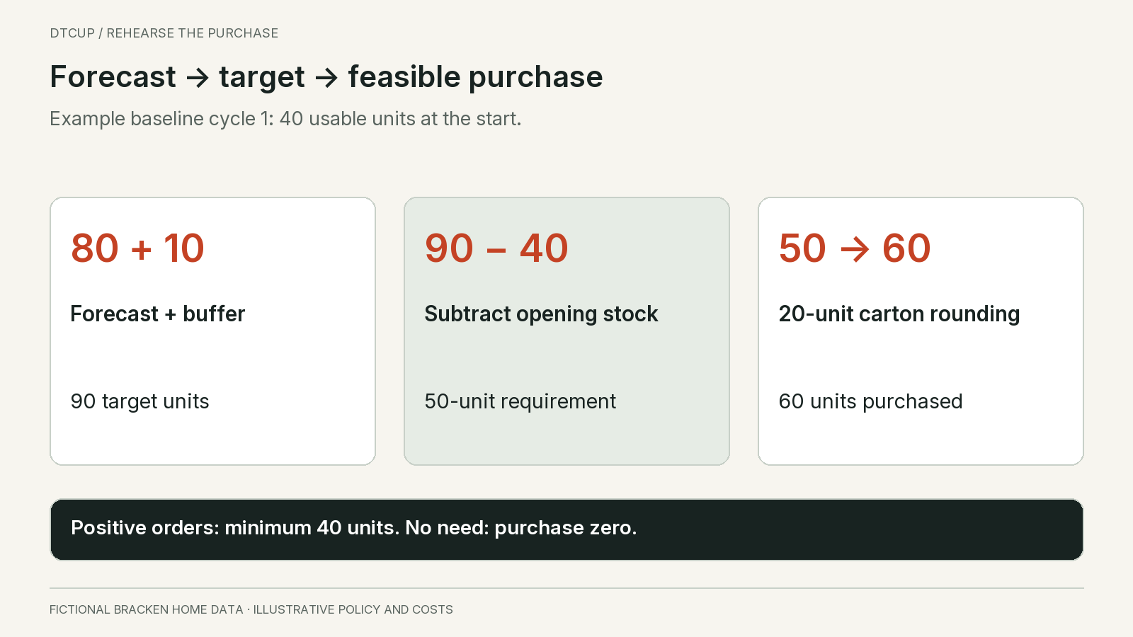
The target available quantity is the forecast plus a fixed ten-unit buffer. This buffer is an illustrative policy choice, not a statistically calibrated safety-stock recommendation. Required purchase quantity is the target minus usable opening stock, floored at zero. A positive purchase must be at least 40 units and is rounded upward to a multiple of 20.
In the first baseline cycle, the target is 80 plus 10, or 90 units. Subtract the opening 40 and the unrounded requirement is 50. The 20-unit carton rule raises the purchase to 60. Available stock becomes 100. Actual demand is 80, so the cycle ends with 20 units.
Carry those 20 units into the second cycle. The baseline forecast is again 80, so the target remains 90. The unrounded requirement is now 70, rounded to 80. Available stock is 100 and actual demand is 100. Ending stock is zero. Resetting opening stock to 40 here would be a different experiment.
Under the candidate, the first forecast is 90, making the target 100. The purchase is still 60 because opening stock is 40. Both forecasts therefore produce the same first purchase despite differing by ten units. This is why forecast improvements do not translate one-for-one into changes in actual orders.
In candidate cycle two, opening stock is 20 and the forecast is 105. The target is 115, the unrounded requirement is 95 and the purchase rounds to 100. Available stock becomes 120. After 100 units of demand, 20 remain. Now the forecasting difference has crossed a carton boundary and changed the decision.
Apply the same buffer, minimum and rounding rule to both methods. If you change the buffer for only one, the comparison is between forecast-policy combinations. That may be the right business comparison later, but label it honestly. First isolate what the forecast changes under a common policy.
7. Carry inventory forward and reconcile the simulated units
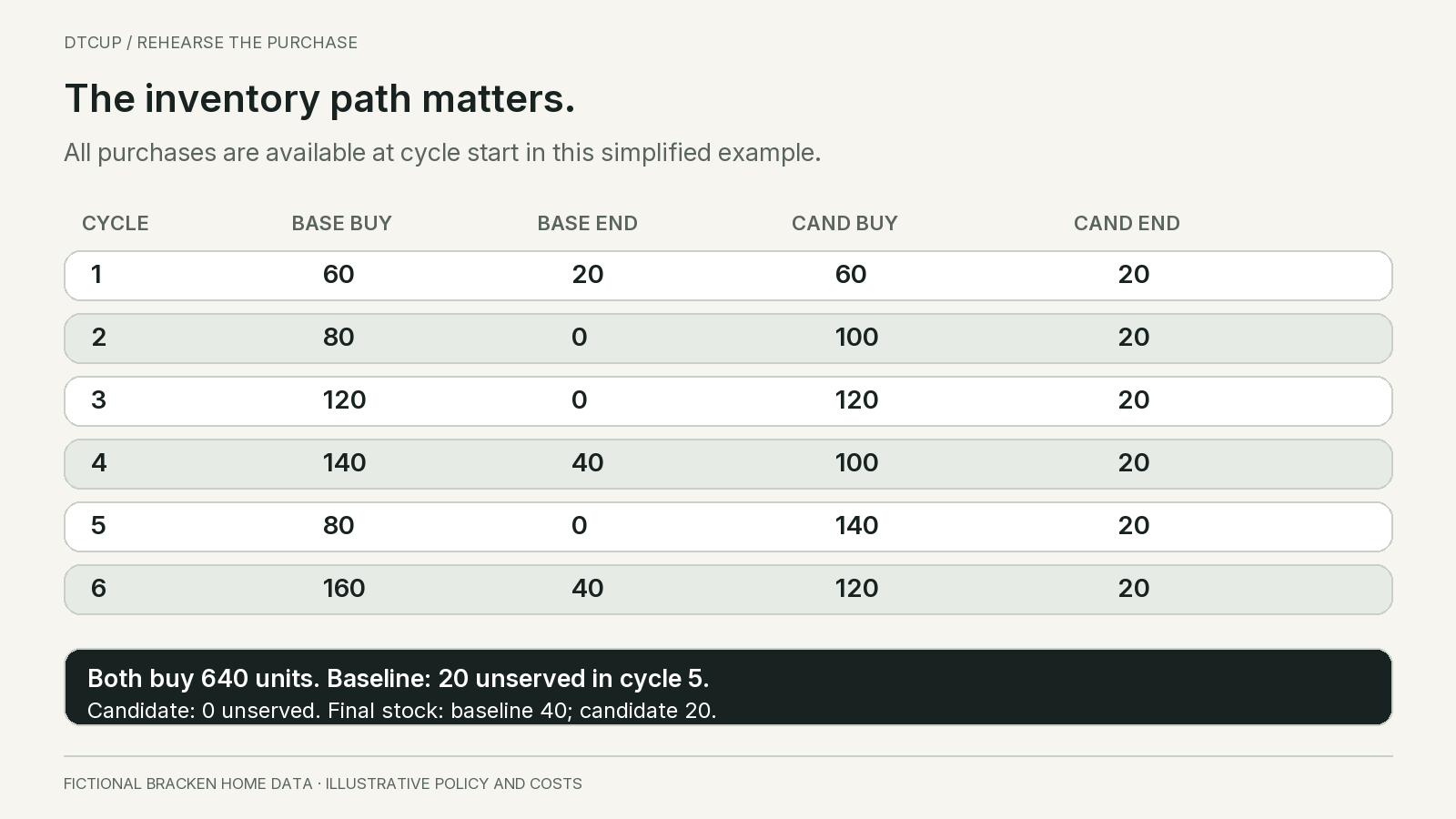
Continue the baseline simulation across all six cycles. The purchases are 60, 80, 120, 140, 80 and 160 units. Ending usable stock is 20, zero, zero, 40, zero and 40. In cycle five, available stock is 120 against demand of 140, so 20 units are unserved in this example.
The simulation assumes those unserved units are lost rather than carried as backorders. That matters. If customers wait and the orders remain open, the next cycle must include that obligation explicitly. Do not switch between lost sales and backlog accounting according to which produces a better-looking result.
The candidate’s purchases are 60, 100, 120, 100, 140 and 120 units. It ends each cycle with 20 units and has no simulated unserved demand. Both methods purchase 640 units in total. The difference is timing: the candidate makes more of that stock available before the high-demand cycle instead of leaving a larger balance at the end.
Reconcile the whole path. Both start with 40 units and buy 640, giving 680 units of supply. Total demand is 660. The baseline serves 640, loses 20 and ends with 40. The candidate serves all 660 and ends with 20. Supply equals served units plus ending stock in both cases, because this simplified example has no shrinkage, returns or other stock movements.
Notice that summing ending inventory across cycles is not the same as counting distinct unsold units. The same physical unit may appear in several ending balances. That sum can support a defined period-based carrying proxy, but it is not a statement that the business has 100 or 120 separate unwanted units at the final date.
Check the intra-cycle assumption before applying the result elsewhere. Because all supply is available at the start and no stock arrives later, the cycle total can determine whether demand is served in this simplified model. With dated receipts during the cycle, a weekly or daily inventory path is necessary; enough stock in total may still arrive too late.
Keep forecast scoring and inventory simulation as separate outputs. The first explains prediction error. The second explains the consequences of a particular policy under a particular supply and demand scenario. A forecast method does not own every result produced by an unrealistic lead-time assumption or an arbitrary purchase constraint.
8. Price the tradeoff without inventing financial certainty
Units alone do not decide the business preference. A shortage can lead to a lost contribution, a delayed order, expedited shipping, a substitute purchase or no lasting loss at all. Ending inventory may sell next period, require a markdown or become obsolete. Use clearly defined consequences instead of calling every unserved unit a lost sale at full retail revenue.
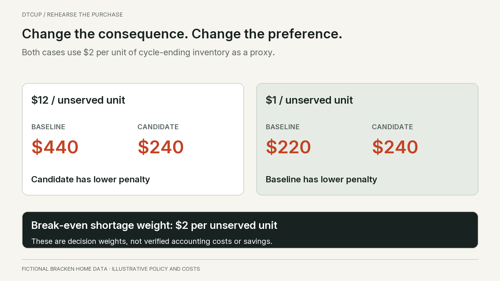
For the teaching comparison, assign a penalty of 12 dollars per unserved unit and two dollars per unit of cycle-ending inventory. These are hypothetical decision weights. The ending-inventory charge is a deliberately simple proxy applied at each cycle boundary, not a claim about actual warehouse or finance accounting.
The baseline has 20 unserved units and ending balances that sum to 100 unit-cycles. Its score is 20 times 12 plus 100 times two, or 440 dollars. The candidate has no unserved units and 120 unit-cycles of ending inventory, giving a score of 240 dollars. Under these particular weights and assumptions, the candidate has the lower penalty.
Now lower the unserved-unit penalty to one dollar while keeping the two-dollar inventory proxy. The baseline score becomes 20 plus 200, or 220 dollars. The candidate remains at 240. The preference reverses even though the candidate’s forecast error remains lower. This is a sensitivity demonstration, not a recommendation to value a disappointed customer at one dollar.
The break-even unserved-unit penalty is two dollars in this constructed example. The candidate adds 20 unit-cycles of ending inventory, costing 40 dollars under the proxy, while avoiding 20 unserved units. Forty divided by twenty is two. Above that weight the candidate wins this simplified score; below it the baseline wins.
Do not combine overlapping penalties without checking. If a shortage penalty already includes expected lost contribution, adding the entire retail price again would double-count the consequence. If an inventory penalty includes expected disposal loss, separately charging the full purchase cost of every remaining unit may do the same. Ask finance to define the actual basis.
Cash commitment is another view, not automatically another expense to add. Both examples buy the same total units, but payment timing differs. A supplier deposit or a limited purchasing budget can make an otherwise attractive sequence infeasible. Show the cash path separately and use actual commercial terms when they are known.
Where the shortage consequence is uncertain, ask which customer response would change the preference. If most buyers wait without canceling, delayed-service cost may be more relevant than lost contribution. If a missing component prevents a larger bundle order, the consequence may exceed the standalone item’s margin. Record those mechanisms and estimate them from appropriate evidence rather than applying one penalty across unrelated products.
A useful review can therefore end with a threshold instead of one supposedly precise dollar result: the candidate is preferred only if avoiding an unserved unit is worth more than the calculated break-even amount under the other stated assumptions. That gives the buyer a concrete evidence question to resolve.
9. Add real constraints in an order that preserves understanding
Once the simple simulation reconciles, add the conditions that materially affect the actual purchase. Lead time should usually come early. Stock ordered today cannot serve yesterday’s shortage, and a receipt expected next month should not appear in this week’s available balance. Model the date stock becomes usable, including receiving or inspection where relevant.
Separate known commitments from new decisions. An open purchase order at the historical origin may already be binding. A forecast change does not automatically cancel it. Include the agreed quantity and the information about its expected timing that was available then. Do not replace that expectation with the eventual actual arrival before the simulation reaches it.
Use alternative receipt scenarios when timing was uncertain. For example, compare the recorded expected date with a plausible delay supported by the business’s own history. If the preferred forecast-policy combination only works under perfectly punctual supply, the result should say so. Avoid assigning precise receipt probabilities without evidence.
Add cash or capacity constraints explicitly. A model that recommends purchases beyond the available budget is not an executable plan. Decide how the simulated buyer allocates limited funds before seeing later demand. Otherwise the simulation can quietly direct cash to the products that hindsight reveals were most valuable.
Keep shelf life and product change visible. Ending stock that remains useful is different from inventory that will be obsolete after a redesign. If the simulation charges an ending balance as though it retains full value indefinitely, it may favor overbuying. If it writes off every final unit immediately, it may unfairly punish a sensible continuing-stock position.
For several locations, include transfer time and destination availability. Business-wide stock cannot satisfy a local promise instantly. Likewise, product substitutions should be governed by an explicit rule and a defensible demand assumption. Do not assume every customer accepts the available alternative simply because it makes the simulated service rate higher.
Add one meaningful layer at a time and inspect how the decision changes. The purpose is not to build the most elaborate simulator. It is to identify which assumptions control the recommendation and whether those assumptions describe the business closely enough to support a purchase.
Consider a separate timing example with sixty units available initially and sixty more arriving at the beginning of week three. Total four-week demand is 120. If weekly demand is 30, 30, 30 and 30, the initial stock covers the first two weeks and the receipt covers the last two. If demand is 50, 40, 20 and 10, the same total supply leaves thirty units unserved before the receipt under a lost-sales assumption.
In the second path, the first two weeks consume sixty and leave thirty units of demand unserved. The receipt then supplies sixty against only thirty remaining demand, leaving thirty units at the end. An aggregate calculation of 120 supply minus 120 demand would incorrectly suggest a perfect match. This is why a realistic backtest must preserve the timing resolution needed by the promise.
Do not automatically move that missed demand into later weeks. Some customers may wait, some may substitute and some may leave. Each behavior produces a different inventory path. When the evidence cannot distinguish them, show scenarios and label the assumption rather than making the forecast appear accurate by changing the demand after the shortage.
10. Avoid selecting a winner that only wins the historical contest
Trying enough models, windows, buffers and exclusions will usually produce an attractive historical result. That does not mean the selected combination will perform similarly next month. The more decisions you make after seeing the outcomes, the more important it becomes to preserve an untouched evaluation period and document the selection process.
Choose a small, reasoned candidate set. A recent-value baseline, an appropriate seasonal reference and one more structured method can answer more than dozens of unexplained variants. Record why each candidate could improve the relevant demand pattern. A method should have a hypothesis, not just a fashionable name.
Separate forecast tuning from purchase-policy tuning. You might first compare predictions under one fixed policy, then compare a few policy alternatives for a shortlisted forecast. If you optimize both simultaneously, the winning configuration may be difficult to interpret and unstable. There are legitimate joint optimization methods, but the small-team review still needs to know what changed.
Inspect performance across different operating conditions. A candidate may help during stable demand and fail around promotions. Another may work for established products but react badly to launches. That can justify scoped use rather than a universal winner. Do not assign a model to a product group based on an outcome you could not have known at the assignment date.
Keep bad periods in view. Removing every disrupted week because it seems unusual creates a backtest for a business that never faces disruption. Some periods may be excluded for a specific valid reason, such as a missing source or a product that did not yet exist. Record the reason and show how the conclusion changes when relevant uncertainty is restored.
Be cautious with small improvements. Bracken has only six nonoverlapping cycles in the teaching example, so its result is descriptive. It does not establish a stable ranking across seasons or products. In real work, assess how much evidence supports the apparent gain and whether the gain survives reasonable changes to assumptions.
Keep an operational fallback. A method that performs well historically but requires unavailable inputs every Monday may be less useful than a simpler method the team can run reliably. Compare data freshness, maintenance effort and failure behavior alongside the simulated outcome. A forecast nobody can produce on time cannot improve that day’s order.
Define the end of the simulation before looking at the winner. Inventory remaining on the last day still has a future. A short test ending immediately after a large receipt can make a reasonable replenishment look wasteful; ending just before the receipt can hide the commitment altogether. Report final usable stock, open orders and unpaid commitments alongside the scored period, and consider a longer follow-through window when those balances dominate the result.
Similarly, define how newly introduced and discontinued items enter the comparison. Requiring a long uninterrupted history can exclude the exact products that create the hardest purchase decisions. Keep mature-item model selection separate from launch and retirement planning rather than quietly dropping those items from the business-level conclusion.
11. Give the buyer a review record, not just an accuracy chart
The final comparison should state the purchase question, demand scope, origins, forecast horizon, data cutoffs, methods, policy and constraints. It should then show prediction errors, simulated stock outcomes and consequence assumptions separately. A reviewer should be able to follow the chain from historical information to the proposed purchase rule.
Include the worst relevant decisions. Which cycles ran short? Which accumulated stock? Which required a purchase that breached the assumed budget? Showing these cases allows the buyer to challenge the business logic. A single score cannot reveal whether the method’s weakness occurs exactly when the business is least able to absorb it.
Include a simple arithmetic acceptance check as well: opening stock plus usable receipts minus served demand and other documented outflows must reconcile to closing stock. New purchase orders should appear once, and their receipts should not be counted again as fresh decisions. A small reconciliation difference can indicate a much larger logic problem when repeated across hundreds of items.
State which inputs were truly historical and which were reconstructed. If inventory snapshots were unavailable and opening balances were estimated, say that the purchase simulation is approximate. If only aggregate demand was available, do not claim to have tested intra-week availability. Precision in the output table should not exceed precision in the underlying evidence.
For Bracken, a defensible conclusion is that the constructed candidate has lower mean absolute forecast error and better simulated service under the stated common policy. Its penalty advantage depends on the chosen shortage weight, and the simulation assumes immediate cycle-start availability. That conclusion is useful because it includes the conditions under which it holds.
An indefensible conclusion would be that the candidate will save 200 dollars every six cycles or eliminate stockouts. The 200-dollar difference is produced by invented weights and demand in a teaching example. A real result would still depend on future demand, execution, supply and whether the test’s assumptions remain valid.
End the review with an explicit next step. That might be to collect missing lead-time snapshots, test a later untouched period, use the candidate for a bounded product group in shadow planning or keep the baseline. Record who owns the next step and what evidence would change the decision. Do not translate a favorable backtest directly into unattended purchase orders.
For products with little history, use the separate first-reorder framework. A long-looking spreadsheet cannot create mature seasonal evidence for a new product. In that situation, scenario planning and limited commitments may be more defensible than declaring a statistically superior model.
12. Turn historical evidence into a measured operating change
Begin with shadow decisions where practical. At each real review, save what the current process would buy and what the candidate process recommends, using the same information cutoff. The buyer can compare the rationale without immediately changing the commercial commitment. This also tests whether the required data and calculations arrive in time.
When the candidate influences an actual purchase, preserve the override history. If a buyer changes the quantity because of a supplier notice, record the notice and timing. Later, distinguish the model recommendation from the executed order. Otherwise success may be credited to a forecast that the buyer ignored, or a failure blamed on a quantity the model never recommended.
Review outcomes after the relevant demand and supply periods have matured. A recent order cannot yet reveal the full effect of a long replenishment cycle. Track immediate execution issues separately from eventual service, inventory and financial outcomes. Avoid announcing success simply because the purchase file was generated without an error.
Maintain a simple fallback when data becomes stale or a required input disappears. The fallback might be the approved baseline plus manual review for affected items. It should be visible as a degraded process, not silently presented as a fresh candidate forecast. The buyer needs to know which evidence supports the current recommendation.
Keep updating the historical rehearsal as new periods become available, while preserving earlier results. A model can become less useful after a pricing change, assortment shift or new channel. Re-evaluation should distinguish a changed business from a defective implementation, and should not rewrite the past to make the latest choice look inevitable.
The practical standard is straightforward: use information available at the decision time, forecast the period the purchase must protect, apply an executable policy and examine the consequences. The best forecast for the business is the one that supports a defensible decision under its constraints, not necessarily the one with the most impressive chart or the most complicated name.
Sources
Still have a question?Ask the DTCUP Community ↗