
Sales Are Not Demand: Build the Right History Before Forecasting
Orders, shipments and refunds can produce different totals without any of them being wrong. Reconstruct a fictional SKU ledger and define the history your replenishment decisions actually need.

7 years of experience building and operating brand websites, specializing in website development, paid advertising and SEO. Built a brand website from launch to US$10 million in annual sales.
The Short Answer
Start with an explicit eligible ordered-unit definition and keep shipments, refunds, cancellations, availability and service replacements separate. Reconcile the source at line level, preserve event dates and coverage limits, and distinguish observed orders from estimated unconstrained demand.
Key takeaways
- Customer orders, warehouse shipments and refunds answer different operational questions.
- A refund does not automatically return a sellable unit to inventory.
- Supply-related cancellations can indicate unmet demand, but adding them back requires checking later reorders and substitutes.
- Missing source data, unavailable stock and a genuine zero must remain distinguishable.
- Connect existing obligations and expected new orders in a fulfillment plan without counting either twice.

A buyer asks how many units sold last month. Finance says 47. The warehouse says 41. The order export appears to show 96. The forecasting sheet uses 60. Before anyone replaces the software, it is worth asking whether these numbers describe different events rather than different versions of the truth.
Inventory planning starts with a definition of the demand you want to serve. An order records a customer’s commitment under the conditions offered. A shipment records fulfillment. A refund records a financial adjustment, sometimes linked to returned goods and sometimes not. A stockout can prevent an order from appearing at all. Combining these signals without preserving their meaning can make the next purchase decision confidently wrong.
I would build a transparent demand history before choosing a forecast model. Keep the original events, define an eligible order-unit series, and retain cancellations, refunds, availability and service replacements as separate evidence. That gives the team a way to explain both the number and its limitations. It also makes later forecasting experiments comparable because they begin with the same question.
This article uses a fictional desk-accessory brand and one fictional SKU, TM-400. All quantities, order references and operating situations are invented teaching data. We will reconstruct a small period, explain why several totals can be legitimate, and turn the result into a data specification a buyer and analyst can agree on. The goal is a usable planning history, not an accounting policy or a claim that recorded orders reveal all potential demand.
1. Define the planning question before choosing the sales field
The word demand can refer to several things. Commercial demand concerns what customers seek to buy. Warehouse workload concerns what must be picked and shipped. Component demand concerns the parts required to assemble offers. Net retained sales concern purchases that remain after relevant adjustments. These quantities interact, but they are not interchangeable planning targets.
For replenishing a finished product sold on a website, eligible ordered units are often a useful starting signal. They place the event near the customer’s buying decision rather than the warehouse’s dispatch schedule. However, the eligibility rule must be explicit, and orders remain constrained by stock, availability, price, traffic and the offer. Calling the series observed order demand is clearer than pretending it is unconstrained market demand.
Write the decision in one sentence. For TM-400, it might be: estimate future customer order units so we can review replenishment before sellable stock runs short. This differs from estimating next week’s packing workload, which also needs the existing backlog and fulfillment schedule. It differs again from estimating cash receipts, which needs prices, payment timing and refunds. A single dashboard field should not silently serve all three purposes.
Choose the unit and grain at the same time. One product unit, one pack and one order are different quantities. A ten-pack sold as one line item may consume ten physical components. An order containing three products should not become three orders. Start with the smallest stable business object needed for the decision, usually a product variant or SKU in a defined store or channel, then aggregate deliberately.
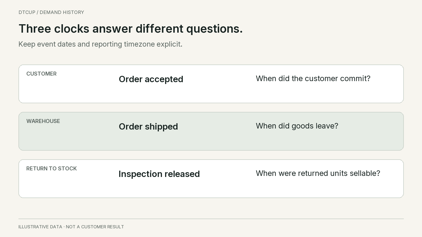
Agree on the event date. For order demand, use the chosen order event in the business’s reporting timezone. For shipment workload, use the fulfillment event. For returned-stock availability, use the inspection or sellable-release event rather than merely the refund date. These choices determine the shape of the time series. A delay in shipping should not automatically move the customer’s original demand into a later week.
Also name the exclusions before inspecting the result. Test orders, duplicated export rows, unconfirmed transactions and service replacements may need different treatment. The exact rule depends on the business process. The important requirement is that the series has a stated definition, and excluded records remain explainable. “We removed the strange rows” is not a reproducible planning method.
2. Reconstruct the period from individual order lines
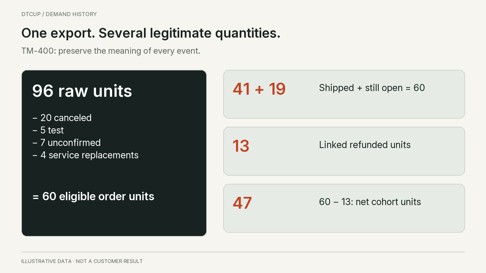
Our fictional export contains ten TM-400 lines totaling 96 units. Order A100 has 20 paid units, all shipped, with four units later linked to a refund. A101 has 12 units canceled after the customer changed their mind. A102 has eight units canceled because the business could not supply them. A103 has 15 eligible preorder units, none shipped yet. A104 has ten eligible units, six shipped and four still open.
The remaining lines have different meanings. A105 contains five test units. A106 contains seven unpaid, unconfirmed units that the business does not treat as accepted demand. A107 has nine eligible units, all shipped and later refunded after a return. A108 is a four-unit no-charge service replacement. A109 has six eligible units, all shipped. There are no duplicate rows in this first example.
For this teaching series, the agreed commercial order definition excludes the 20 canceled units, five test units, seven unconfirmed units and four service-replacement units. The eligible total is 96 minus 20 minus five minus seven minus four, which equals 60. That is a defined observed-order series. It does not claim the eight stockout cancellations represented no customer interest; they remain a separate unmet-demand signal.
The eligible commercial shipments total 41: 20 from A100, six from A104, nine from A107 and six from A109. The remaining eligible open quantity is 19: 15 from A103 and four from A104. Therefore, for these simplified records, 60 ordered units reconcile to 41 shipped plus 19 still open. The four service replacements are additional physical workload, but they are not new commercial purchases in this definition.
The line-linked refunded quantity is 13: four from A100 and nine from A107. Subtracting those from the 60 eligible order units gives 47 net order units under this deliberately simplified cohort measure. That explains finance’s possible quantity view, but it does not mean only 47 units created replenishment needs. Some refunded products may be damaged, unavailable for resale or still in transit back to the business.
Now the opening numbers make sense. Ninety-six is raw export quantity. Sixty is eligible commercial order quantity. Forty-one is the shipped quantity from that eligible cohort. Forty-seven is a net quantity after the specified line-linked refunds. None should be labeled simply “sales” without context. The correct input depends on the decision, and each total needs its own reconciliation.
In a real dataset, this simple identity needs adjustments for partial cancellations, exchanges, order edits and other events. Do not force messy records to fit the example by deleting inconvenient rows. Use the example to establish the principle: preserve the event meanings, document the eligibility rule, and explain the difference between totals before fitting a model to one of them.
3. A refund does not rewind the customer’s original demand
A customer can genuinely want a product, receive it, and later request a refund because it arrived damaged. The refund changes the financial outcome. It does not prove that the original demand never existed. If a forecast subtracts every later refund from the original units without considering the reason and physical outcome, it can learn an artificially low demand signal.
The opposite mistake is ignoring returns completely. High returns may reveal a product problem, misleading content, incorrect sizing or customers ordering several variants to keep one. That information should influence the business plan and may justify a separate net-retention forecast. The point is to preserve it as a meaningful signal rather than bury it inside a number whose purpose is to estimate incoming order units.
In the fictional example, A100’s four refunded units and A107’s nine refunded units have different possible operational consequences. A financial refund may happen without a physical return. A returned product may need inspection. Only units that are actually fit for resale and released into sellable inventory should reappear as usable supply. A refund event by itself is not an inbound stock receipt.
Keep at least three quantities distinguishable: refunded item units where linkage exists, physically returned units, and returned units released for resale. Do not invent item quantities from a money-only adjustment. A partial goodwill refund may not correspond to a fraction of a physical product. If the source cannot establish the quantity, label the limitation instead of dividing the refund amount by the current selling price.
Timing matters as well. A refund recorded in October may relate to a September order. A report grouped by refund date answers a different question from a report that revises the September order cohort. Both can be useful, but the labels and comparisons must explain the date basis. Otherwise the team may interpret a week of processed returns as a sudden collapse in new customer demand.
For replenishment, I would begin with the agreed eligible order signal and model return-to-stock separately when its timing and quality are dependable enough to matter. For financial planning, use the appropriate revenue and refund definitions with the responsible finance owner. For product improvement, examine reasons and repeat patterns. One subtraction should not replace these three different decisions.
Exchanges deserve particular attention. An exchange can create an outgoing replacement and an incoming return without representing a wholly new independent purchase. Link the exchange where the source supports it, preserve the physical movements, and decide whether the planning target is initial choice, retained choice or warehouse workload. Counting every exchange shipment as fresh market demand can exaggerate the popularity of products with high exchange rates.
4. Cancellations can mean lost interest or unmet demand
A canceled order is not one uniform event. A customer who changes their mind before confirmation provides different evidence from a customer whose paid order is canceled because the product cannot be supplied. A fraud cancellation differs from a duplicate order. If all canceled quantities are either fully included or fully erased, the planner loses these distinctions.
Our base series excludes canceled commercial lines so its definition is stable and easy to reconcile. Alongside it, we retain cancellation quantity and reason. A101’s 12 changed-mind units are not automatically added back as future demand. A102’s eight supply-related cancellations are evidence that observed completed orders may understate interest. Even then, adding all eight to a forecast without checking the circumstances would be an assumption, not an observation.
Ask whether the customer bought a substitute, reordered later, or appeared in another channel’s records. A stockout cancellation followed by a successful order of the same item should not be counted twice when estimating the underlying need. Conversely, an abandoned attempt that never became an order may not appear in cancellation data at all. The cancellation ledger is a partial view of unmet demand, not a complete measurement of it.
Partial cancellations should be handled at the line and quantity level where possible. If an order originally requested ten units and two were canceled, the remaining eight still matter. An order-level canceled flag can be too coarse for edited or partially fulfilled orders. Confirm what the provider’s fields mean and retain the original and revised quantities needed to reconstruct the state.
There is also an as-of problem. An order was open when a forecast was made but canceled two weeks later. A current export may show only the final state. If you use that final state when backtesting the earlier forecast, you may be giving the historical model information that was unavailable at the time. Keep event history or saved dataset versions where practical, and disclose when an evaluation uses retrospectively cleaned data.
This does not mean the business must build a complex event platform before forecasting anything. It means the planner should know whether the history represents what was known then or what is known now. Start with a clear current-state reconstruction, record its limitations, and improve the history where the difference changes purchasing decisions. Hidden hindsight is more dangerous than an openly limited baseline.
5. Keep the customer clock separate from the warehouse clock
Shipping history is tempting because it often looks concrete: units physically left the building. But shipment timing also reflects stock availability, staffing, weekends, batching and carrier collection. A warehouse backlog can turn several days of steady orders into one large dispatch spike. Forecasting future customer demand from that spike may teach the model the warehouse’s schedule rather than the customer’s buying pattern.
For A103, the 15 preorder units are observed commitments in the order period under our agreed eligibility rule. They are also future fulfillment obligations. They should not be treated as 15 units of fresh demand again on the day they ship. A workload plan can include them on the expected dispatch date, while a demand history retains their original order timing.
Preorders need a clear label because they change what availability means. A product can accept orders while having no sellable stock today. That differs from an ordinary stockout where checkout is disabled. The customer promise, cancellation behavior and backlog may all differ. Keep the offer type and expected fulfillment timing visible rather than mixing preorder and immediate-delivery demand without explanation.
Use the business’s reporting timezone consistently. An order near midnight UTC may belong to the previous local date. Mixing UTC order buckets with local warehouse buckets can create daily mismatches that look like missing units. Record the source timestamp, the chosen business timezone and the derived reporting date. Avoid manually shifting dates in a spreadsheet without preserving the rule.
Compare complete periods. A month with only ten synced days is not a full month of low demand. A current day halfway through its trading hours is not directly comparable with a completed day. When the source coverage is partial, label it and choose an appropriate comparison or decline to calculate one. A percentage can be mathematically computable while still being operationally misleading.
For planning meetings, I would show ordered units, shipped units and open eligible units side by side for a clearly defined cohort, then show a separate dispatch-date workload view. This makes it easier to see whether the issue is demand growth or execution delay. The two views should connect, but forcing them into one time series makes both harder to interpret.
6. Separate zero demand, missing data and constrained sales
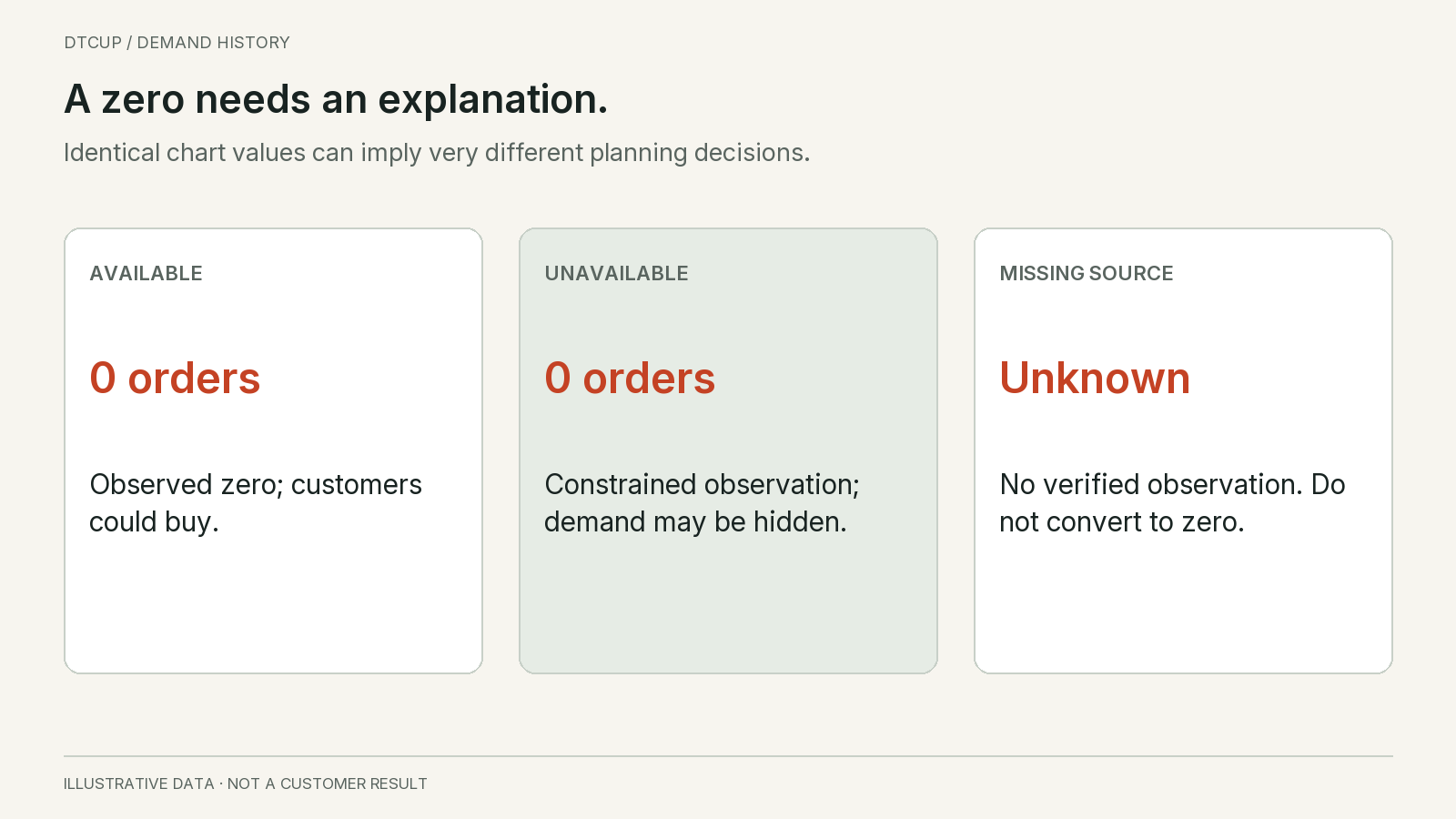
A row containing zero can mean several things. The product was available and nobody ordered it. The product was unavailable and customers could not order it. The store was closed. The data connection failed. The SKU did not exist yet. Treating all these states as equivalent tells the forecast a story that the underlying records do not support.
Build a complete date grid for each planning item, but attach a coverage state before filling gaps. If the source is complete and the product was offered, a missing order row may legitimately become zero observed orders. If the source did not sync, leave the quantity unknown. If the product was not yet launched, distinguish that from an ordinary zero-sales day after launch.
Availability deserves its own observation. In a three-day fictional sequence, Monday has complete data, available stock and zero orders. Tuesday has complete data but checkout disabled for the item. Wednesday has an incomplete order sync. The first is an observed zero under available conditions. The second is constrained exposure. The third is unknown. A neat row of three zeroes would erase the difference.
The forecasting text Forecasting: Principles and Practice discusses missing values and unusual observations as context-dependent problems. The relevant lesson is to investigate why a value is missing or unusual before replacing it. For an inventory series, that investigation includes whether the business could actually accept the order and whether the source covered the whole period.
Do not assume stockout demand is zero, and do not assume it equals the average from surrounding days. A promotion, traffic change or substitute product can make the surrounding period different. Record any estimated lost demand separately from observed orders, with the assumption and method visible. The later forecast can compare scenarios without rewriting the original history as if an estimate were an observed sale.
Current stock does not prove historical availability. If the warehouse has stock today, that says little about whether the item was purchasable last Tuesday. Historical availability may require inventory observations, website availability events or another trustworthy source. When that history is absent, say that stockout correction is uncertain. Do not reconstruct exact unavailable hours from a current inventory snapshot.
For a first planning baseline, a visible limitation is better than a hidden correction. Flag the affected periods, inspect how much of the history they represent, and compare the purchasing decision under plausible assumptions. If most of the product’s short history was constrained or missing, the team may need a launch-style scenario rather than a confident time-series forecast.
7. Map the item the customer buys to the item the business must replenish
A product title is not a dependable planning key. Titles change, translations differ, and several variants can share most of their wording. Use stable source identifiers and a reviewed mapping to the merchant’s planning SKU. Keep store and channel scope in that mapping so identical-looking codes from unrelated catalogs are not silently combined.
Missing and duplicate mappings should create an exception, not an automatic guess. If two variants both map to TM-400, confirm whether they truly represent the same replenishable item. If one variant changes its physical contents while retaining a familiar title, the historical series may need a version boundary. A forecast cannot distinguish a product redesign from a demand change unless the data carries that information.
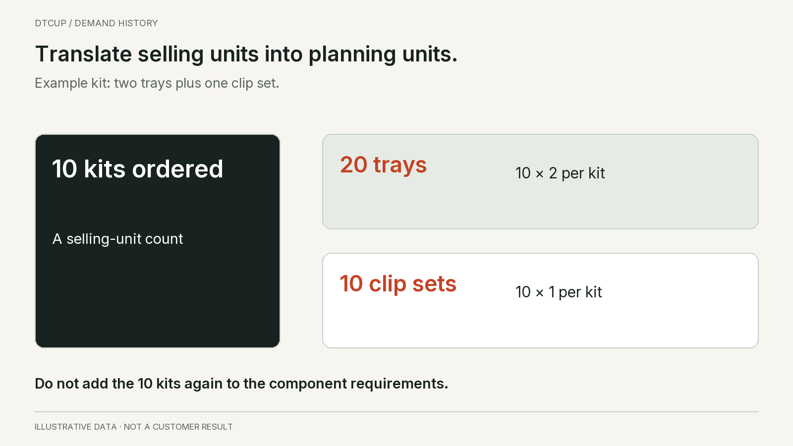
Bundles create another layer. Suppose the website sells a kit containing two trays and one set of clips. Ten kit orders imply twenty trays and ten clip sets for component planning, assuming that is the approved bill of materials. The website’s ten sellable units and the warehouse’s thirty component units are both legitimate, but adding them together would double-count the same commercial activity.
Keep commercial demand and component requirements as linked views. The commercial view helps understand the offer customers choose. The component view helps replenish the items consumed by that offer. If components also sell individually, combine their direct demand with the bundle-derived requirements only after applying the correct quantities and effective product configuration. A kit change should not rewrite old orders using today’s component recipe.
Multipacks require equally explicit conversion. One two-pack and two single units may consume the same number of physical products but have different packaging needs and customer behavior. Decide whether the planning item is the packaged unit, the underlying component or both. Record conversion factors with their effective scope rather than hiding them in a spreadsheet formula nobody remembers updating.
Service replacements should enter the physical requirement plan separately. A108’s four replacement units consume stock even though they are excluded from new commercial order demand. If replacement demand is recurring and material, estimate it as a service requirement with its own driver, such as the relevant installed base or observed replacement pattern. Do not pretend it is free simply because it has no sales revenue.
Use a small reconciliation sample before relying on the mapping at scale. Pick a normal variant, a bundle, a multipack, a changed product and a replacement order. Trace each from the source line to the planning quantity. This is a much more useful early check than comparing only the grand total, because two opposite mapping errors can cancel each other in an aggregate report.
8. Handle duplicates and edits without manufacturing movement
Data imports can repeat the same order line after a retry or an incremental refresh. If each arrival is treated as new demand, a healthy sync process can create an unhealthy forecast. Use a stable source identity for the order and line, scoped to the correct store, and distinguish an updated record from a new event.
Do not deduplicate by product, quantity and timestamp alone. Two genuine customers can buy the same quantity at nearly the same time. Conversely, an edited line can keep its identity while changing quantity. The deduplication rule should follow the source system’s object and event semantics. When those semantics are unclear, investigate a small sample rather than choosing the rule that makes the total look convenient.
Order edits need a defined treatment. If a customer increases an order from two units to three before fulfillment, the system should not count both the original two and the updated three as five independent units. Depending on the planning design, the latest state may represent three total units, while an event history records the additional unit at the edit time. Both approaches need clear labels and reconciliation.
Backfills can also change history. A connection may initially contain only recent orders, then import older records later. A previous zero could become a valid quantity because coverage improved, not because customer behavior changed. Preserve the earliest complete period and the last successful sync information. When a historical total changes materially, identify whether it came from a business event, a source correction or a coverage update.
Make corrections reviewable. Keep the original source reference, corrected interpretation, reason and effective dataset version where appropriate. This does not require retaining unnecessary personal information in the planning table. It requires enough lineage to explain why last week’s forecast input differs from this week’s. Otherwise the team may blame a model for changes introduced by the data preparation process.
A useful acceptance test is idempotence: importing the same source records again should not change the resulting order-unit totals. Another is a controlled edit: increasing one eligible line by one unit should change the relevant total by one under the agreed rule. A third is a linked refund: it should update the refund view without silently deleting the original observed order. These small tests protect the meaning of the series.
9. Keep promotions, price and exposure alongside the quantities
A clean order series still does not explain why customers bought. The same product can sell differently under a discount, a new advertisement, a prominent homepage placement or a delivery promise. Preserve material commercial context so the planner does not interpret every spike as a permanent increase in baseline demand.
Record known promotion periods and offer changes with their actual scope. A sitewide campaign may exclude certain products. A bundle promotion may shift demand away from individually sold components. A price reduction may begin halfway through a day in the reporting timezone. The context should be specific enough to support the decision without pretending every campaign has a measurable, isolated effect.
Separate the observed change from its proposed explanation. “Orders increased during the campaign” is an observation. “The campaign caused all of the increase” requires stronger evidence. Seasonality, availability, channel mix and other changes may contribute. A demand-planning note can preserve those competing explanations and use scenarios rather than assigning an unsupported lift factor to the next purchase order.
Exposure matters for interpreting zeroes and growth. A product removed from navigation may still be technically in stock but receive much less attention. A new marketplace listing may reach a different audience. Website visits can provide useful context, but they are not equivalent to purchase intent, and bot or measurement changes can distort them. Use exposure evidence cautiously and keep its definition separate from order demand.
Large unusual orders should be investigated rather than automatically removed. A wholesale purchase may be real but unlike ordinary retail demand. A one-time project order may not recur next month. Keep the transaction in the appropriate commercial record, then decide whether the recurring-demand forecast should model it separately. Deleting every inconvenient spike can erase valuable information about the business.
I would maintain a short event calendar connected to the SKU history: promotion, price, launch, availability disruption, channel addition and known one-off order. The calendar is explanatory evidence, not a license to fit a detailed story to every fluctuation. Its value is helping the buyer ask better questions before treating the recent average as a stable future rate.
10. Give the demand history a small, explicit data contract
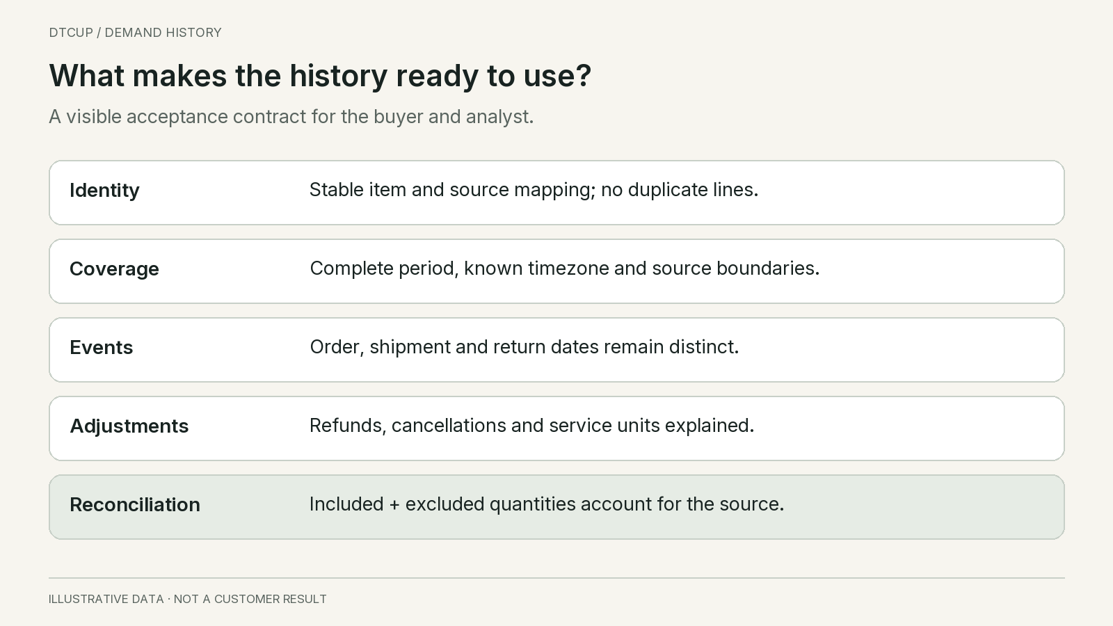
A data contract is simply an agreement about what the table means and when it can be trusted for a particular purpose. For this task, it should identify the planning SKU, source store, reporting date and timezone, eligible ordered units, shipped units, linked refunded units, cancellation quantities and reasons, service requirements, and coverage state. Availability and commercial events can be linked records rather than overloaded columns.
For every quantity, write the inclusion rule and source. State whether the number represents current final state or events known at a historical point. Explain how order edits, partial cancellations and replacements are handled. A plain-language definition beside the table is often more valuable than an elaborate dashboard with ambiguous labels.
Define the conditions that stop automatic use. Missing SKU mapping, incomplete source coverage, duplicate identities, unexplained quantity differences and stale inventory observations should produce visible exceptions. Some may block a forecast; others may permit a clearly labeled limited view. Decide the behavior deliberately instead of letting a blank field become zero through a default formula.
Keep input quality separate from forecast confidence. A model can fit a corrupted series closely and still be useless. A clean short series can be truthful but insufficient for seasonal inference. The interface should allow both statements: the source reconciles, and the forecast remains uncertain. Combining them into one green indicator hides what the buyer actually needs to know.
DTCUP Demand’s current approach uses eligible ordered units before refunds as its demand signal and presents refunded units separately. It also checks complete local-calendar periods before showing the implemented month comparisons. That does not mean every proposed planning feature or warehouse connector is already live. Connection scope, source completeness and available evidence still determine which decisions a particular workspace can support.
If you already use a broader inventory process, connect this contract to the inventory planning method. That guide addresses replenishment and operating decisions. The contract here establishes the history those decisions will rely on. A clear source definition should travel with the forecast rather than disappearing once a chart is drawn.
11. Reconcile a small period before expanding the history
Choose a complete period and a manageable set of items. Start with a straightforward product, then add a product with returns, an edited order, a bundle and a known availability problem. Compare source records with the prepared table using the same date basis and eligibility rule. Do not begin by comparing two dashboards whose definitions are unknown.
Reproduce the fictional reconciliation in your own terms. Raw quantities should be explainable through included quantities and explicit exclusions. Eligible orders should connect to fulfilled and remaining quantities under the chosen state rules, with any other movements identified. Refund quantities should link to source lines where the data supports that relationship. If the source only provides money, the quantity view should admit that limitation.
Investigate differences at the smallest useful level. A ten-unit discrepancy may be one excluded test order, two duplicated lines or a timezone boundary. A percentage difference at the monthly level does not reveal which. Create a short exception list with source references and explanations, then fix the rule or source issue. Avoid manually overriding the final total without correcting the path that produced it.
Ask the buyer and the analyst to review the same examples. The analyst may understand the API fields while the buyer understands why a replacement order exists. Neither perspective alone is enough. A shared review can reveal that a technically valid field describes a different business event from the one the forecasting process intends to measure.
Once the small period reconciles, extend the history and inspect where the assumptions stop holding. Older data may use different product IDs or incomplete refund linkage. A newly connected channel may have partial coverage. Preserve those boundaries rather than stretching today’s definition backward without evidence. A shorter trustworthy history can be more useful than a longer series whose early months mean something else.
12. Use the cleaner history to change the purchasing conversation
Consider how a purchasing review changes when the time horizon is explicit. Suppose the next review covers four weeks, the forecast estimates 55 new eligible order units during those weeks, and the 19 open units in our example must also ship during that period. The gross commercial fulfillment requirement is 74 units before considering service requirements, usable stock and receipts. The 19 are existing obligations; the 55 are estimated future orders. They belong together in the fulfillment plan but should not both be fed back into the historical new-order series.
If four already-approved service replacements must ship in that same window, the physical requirement becomes 78 units. Assume, purely for illustration, that 50 sellable units are available at the start and a confirmed receipt of 20 arrives before those units are needed. That leaves a simple aggregate gap of eight units. This calculation is not a finished purchase recommendation: the receipt may arrive after an early shortage, some inventory may already be reserved elsewhere, and the forecast remains uncertain. It shows why a planning bridge must connect different quantities without pretending they are the same metric.
Now consider the 13 refunded units. Adding all 13 to available stock would erase the apparent gap and create a misleading surplus. If only three have passed inspection and are available before the requirement occurs, only those three can support this particular supply calculation. If those three were already included in the opening 50, adding them again would double-count supply. The correct treatment depends on the snapshot boundary and movement dates, not on whether the refund column happens to be populated.
I would ask the reviewer to walk through this bridge aloud: existing obligations, expected new demand, additional service consumption, usable opening stock, and receipts available in time. Every term needs a date basis and a non-overlapping definition. When a number changes, the team should be able to identify which term changed and why. This is a useful acceptance test for the data preparation work: can another person reconstruct the purchasing discussion without guessing what a dashboard label means? If not, improving the forecast algorithm is premature.
The purpose of this work is not a perfect spreadsheet. It is a better purchasing conversation. In our fictional example, the buyer can now see 60 observed eligible order units, 19 still open, 13 refunded units with separate physical-return implications, four service replacement units, and eight canceled units associated with supply failure. Each points to a different question.
The open units affect near-term fulfillment. The service replacements consume stock without signaling new commercial growth. The refunded units may reveal quality or expectation problems. The supply-related cancellations suggest that observed orders may understate demand, but require deduplication and availability context before adjustment. None of these questions is answered by replacing 60 with 47 and calling the result more accurate.
The next step is to choose a baseline forecast, test it over the relevant purchase horizon and compare plausible demand and supply scenarios. Before doing that, make sure the history says what the team thinks it says. The best forecasting model cannot rescue a series that confuses warehouse timing, refunds, customer choices and missing records.
My recommendation is to keep the observation honest and the interpretation visible. Preserve the orders that happened, the conditions that constrained them, and the adjustments the team chooses to make. Then the forecast can become a reasoned estimate of what comes next, rather than a polished continuation of yesterday’s reporting ambiguity.
Sources
Still have a question?Ask the DTCUP Community ↗