
Stockouts Hide Demand: Estimate the Gap Without Inventing Lost Sales
Low sales during a stockout do not establish low demand. Use a worked tray example to compare available-day baselines, uncertain shortfalls, substitutions, delayed purchases and a concrete expedite decision.

7 years of experience building and operating brand websites, specializing in website development, paid advertising and SEO. Built a brand website from launch to US$10 million in annual sales.
The Short Answer
Keep original orders and availability records separate. Estimate unconstrained focal-SKU demand from comparable available periods, show sensitivity to assumptions, and distinguish substitution and deferred purchases from business loss. Use the estimate to inform future supply decisions without turning it into an automatic backlog.
Key takeaways
- A zero during unavailability is not evidence of zero customer interest.
- Partial-day and variant-level availability change the interpretation of sales.
- The worked flat-rate example estimates 29 missing units, not 29 proven lost orders.
- Unweighted scenarios are not statistical confidence intervals.
- Waitlists, substituted purchases and deferred orders must not be added twice.
- An expedite decision depends on incremental contribution and feasible receipt timing.

A product sells eight units a day, runs out of stock, and then records almost no orders. If the forecast learns only from the order line, it may conclude that demand has collapsed. The next purchase order becomes smaller, the product runs out again, and the business creates a feedback loop in which poor availability teaches the planning system to expect less demand.
The opposite mistake is to fill every stockout day with an optimistic sales number and treat the difference as proven lost revenue. That can inflate the next order, hide weak demand and turn an uncertain estimate into an expensive commitment. A stockout tells you that sales were constrained; it does not reveal exactly how many customers would have bought under different conditions.
I would keep observed orders intact, add a separate availability record, and build a clearly labeled estimate of the demand that might have occurred without the constraint. Then test how the inventory decision changes under different plausible assumptions. The purpose is better replenishment judgment, not manufacturing a precise historical number that the business never observed.
This guide uses a fictional desk tray sold by Alder Supply. All quantities, prices and customer outcomes are invented examples. The method is intended for a brand with limited but usable order and availability data. It is not a claim that a simple average can recover every hidden purchase or that DTCUP has access to a merchant’s unrecorded customer demand.
The statistical issue is often called censored demand: the sales observation is limited by availability. Research such as FreshRetailNet-50K studies this problem using detailed stockout annotations and contextual data. Its setting is fresh retail, so its reported performance should not be assumed for a brand website. The useful lesson here is the need to preserve availability context alongside sales.
1. Decide which missing quantity you are trying to estimate
“Lost sales” can refer to several different things. A customer may have wanted a particular color, bought another color instead, waited for the original to return, purchased from a competitor or abandoned the purchase entirely. Those outcomes have different implications for SKU replenishment, brand revenue and customer experience. One headline number cannot represent all of them accurately.
Start with the narrow planning question: how many units of the focal SKU might customers have ordered during the constrained period if it had been available under otherwise comparable conditions? That is an estimate of unconstrained demand for that SKU. It is not automatically the number of orders the whole business lost.
For Alder Supply, the focal item is the charcoal T-30 desk tray sold on its website. The analysis uses eligible customer order units before refunds, with cancellations and service replacements handled under the defined order-history rules. The sales-to-demand history guide explains why those event definitions must be settled before estimating missing demand.
Keep the planning unit explicit. One tray, one pack of two trays and one bundle containing a tray are not interchangeable counts. If the website sells a bundle, translate it into component demand through the approved bill of materials where that is the planning objective. Do not add bundle counts to single-unit counts and then call the total daily demand for the tray.
Define the channel and market too. A website stockout does not necessarily mean a wholesale partner or marketplace was unavailable. A customer may have bought through another channel, but that should be established through appropriate evidence rather than assumed. The focal estimate might still be useful for website allocation even when total brand demand is partly served elsewhere.
Use three labels in the report: observed eligible units, estimated unconstrained units and estimated shortfall against those observed units. Later, add separate evidence for deferred or substituted purchases. These labels make the uncertainty visible and prevent a modeled quantity from silently replacing the order ledger.
The decision you intend to make should guide the detail. A short shortage before a confirmed replenishment may need a near-term service plan. Repeated shortages during peak demand may justify changes to forecasting and supplier capacity. A one-off discontinued color may need customer communication rather than a new purchase order. Estimate the quantity that informs the actual decision.
2. Build an availability timeline before adjusting any sales
A current inventory balance cannot tell you exactly when the product was purchasable last week. Begin with the best historical evidence available: inventory snapshots, stock-change events, purchase-button status, backorder settings, warehouse release records and known selling restrictions. Record the time zone and the period each observation covers.
For a website, availability is not just physical stock. Units may exist but be reserved, quarantined, inaccessible to the relevant shipping region or blocked by a listing error. Conversely, the site may accept backorders even when immediate physical stock is zero. The planning interpretation depends on what the customer could actually order and what promise the business displayed.
Separate fully available, partially constrained, unavailable and unknown periods. A missing inventory snapshot is not proof of a stockout. A zero closing balance is not proof that the product was unavailable all day. If the last unit sold at 11:50 p.m., most of the day’s demand may have been observable. If it sold at 9:10 a.m., a daily total hides a much longer constraint.
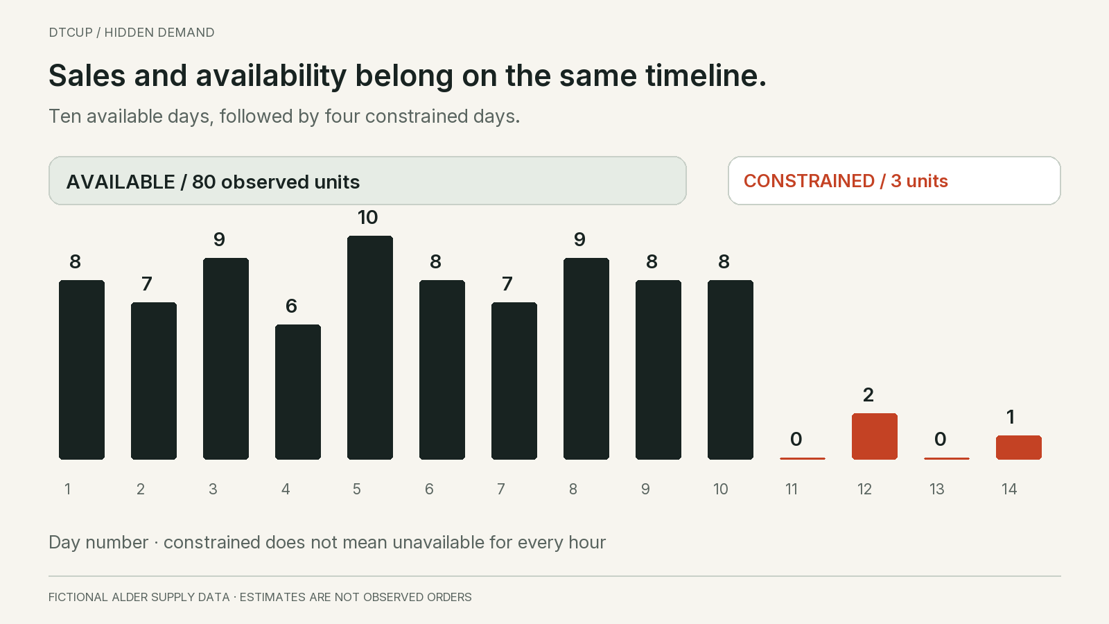
In the fictional example, ten comparison days are verified as available throughout their normal selling periods. Four later days are constrained. Their observed eligible order units are zero, two, zero and one. The small positive counts are possible because limited units became available briefly during those days. We do not relabel all four days as identical full-day stockouts.
Write down the evidence strength for those labels. An hourly stock log is stronger than a staff recollection that the item was “out most of the week,” but even a stock log may not capture a disabled checkout button. If historical information is weak, use a broad scenario and state the limitation. Precision in a spreadsheet does not compensate for uncertain availability timing.
Check whether the constraint was variant-specific. A product page can show an item as available while the popular size or color is sold out. Product-level daily sales may then conceal suppressed demand for one variant and increased sales of another. Preserve the variant identifier and its availability state rather than applying one product-wide adjustment.
Watch for inventory corrections that look like customer demand. A manual stock adjustment, damaged-unit write-off or warehouse transfer can reduce available stock without creating an order. A returned unit may increase physical stock before it passes inspection and becomes sellable. Reconcile those events with their own meanings. The availability timeline should describe the customer’s purchase opportunity; it should not infer orders by subtracting one inventory snapshot from another when non-sales movements are present.
Keep unknown intervals visible until evidence resolves them. Filling a missing stock-status record with the previous day’s state is an assumption, not a recovered observation. Flag it so the sensitivity review can test whether that assumption materially changes the estimate.
Also record changes in exposure. The marketing team may pause ads, remove a homepage placement or stop sending traffic once the product sells out. Those actions are sensible operational responses, but they change the meaning of the counterfactual. Estimating demand under actual reduced traffic is different from estimating demand under the traffic plan that would have continued with stock.
3. Calculate a transparent first baseline
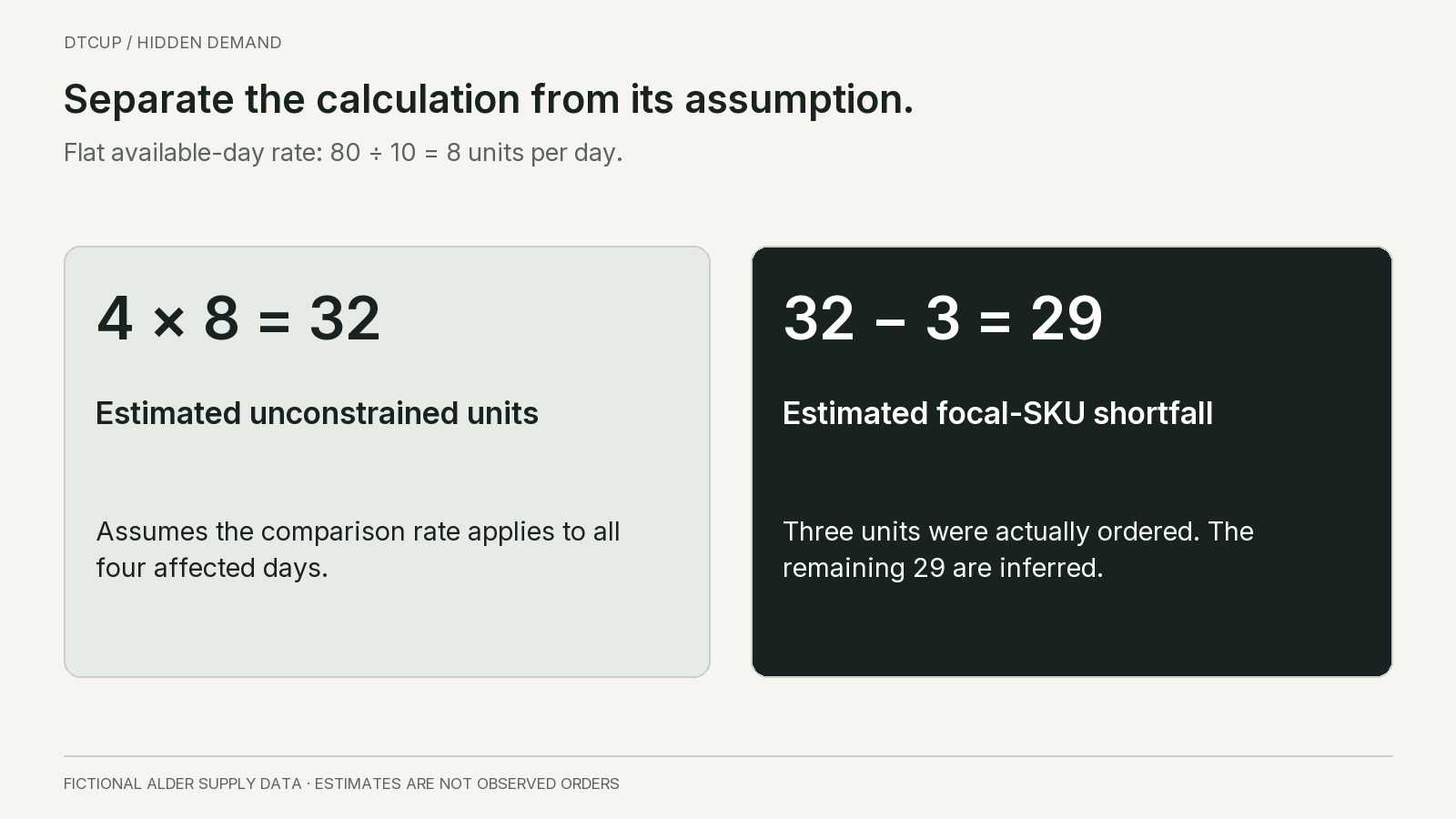
The ten available comparison days for Alder Supply have eligible units of eight, seven, nine, six, ten, eight, seven, nine, eight and eight. They total 80 units, so their descriptive average is eight units per available day. This is a starting reference, not a claim that every future day has demand of exactly eight.
If we apply that simple rate to the four constrained days, the estimated unconstrained total is 32 units. The observed total during those days is three units. The difference is 29 units of estimated unmet focal-SKU demand under the flat-rate assumption. Keep the phrase “under the assumption” attached to the result.
Compare this with the naive average across all fourteen days. Eighty observed units from the available days plus three during the constrained days gives 83. Dividing 83 by fourteen produces about 5.93 units per day. That number accurately describes observed order units across the period, but it is a poor unqualified description of demand when the item was available.
The distinction changes planning. A system using 5.93 as if it were unconstrained daily demand might plan roughly 41.5 units for a seven-day period before other adjustments. A system using eight would start from 56. Neither number is automatically the right purchase quantity, because inventory, open orders, receipts and uncertainty still matter. The comparison simply shows how stock constraints can pull the input rate downward.
Do not overwrite the original 83 units with a reconstructed total and lose the evidence. Store the adjustment in a separate field or analytical layer. A reviewer should be able to recover the original orders, availability labels, comparison set and calculation. If a later review changes the estimate, the accounting and fulfillment records should remain untouched.
Check comparability before trusting the baseline. Were the ten days at the same price, with similar traffic, normal delivery promises and no unusual promotion? Did they include a launch spike or a large wholesale-like order? A clean availability label does not make every day representative. You may need a different comparison set or several alternatives.
Write down why you chose the days. “Most recent available days with unchanged price and normal traffic” is a reviewable rule. “The days that make the forecast look reasonable” is not. If there are too few comparable observations, the honest next step is a broader range or an analogue-based estimate, not an increasingly elaborate average of unsuitable data.
4. Improve the comparison only when the data supports it
A flat daily rate ignores weekday patterns. If the constrained period includes days that normally sell less, eight per day may overstate the shortfall. Suppose a separate set of comparable same-weekday observations suggests six, eight, nine and seven units for the four affected days. The expected total becomes 30, and the shortfall against three observed units becomes 27.
This is not proof that 27 is more accurate than 29. It is a more structured assumption that may be useful if weekday behavior is stable and the comparison data is relevant. Document how many observations support each weekday estimate. A single unusually strong Friday should not acquire authority simply because it shares the same weekday name.
Price and promotion can matter more than weekday. If the stockout followed a discount campaign, the available days during the campaign may not represent normal-price demand. Conversely, removing those days without considering an ongoing promotion may understate what would have happened. Match the estimate to the conditions you are trying to reconstruct.
Traffic-adjusted methods need careful denominators. A conversion rate from available periods can be applied to a comparable traffic measure, but only if the visitor mix, product exposure and purchase opportunity are sufficiently similar. Total website sessions may be a poor denominator when only a subset saw the tray. Product-page visits may themselves fall because the sold-out item was removed from navigation.
Do not automatically divide the few orders received during a partial day by the available fraction of the day. Demand is rarely uniform across every hour. Two orders before a morning stockout do not necessarily imply twice as many orders if availability had lasted twice as long. Use observed intraday patterns only when you have enough comparable information to justify the adjustment.
Be cautious about using neighboring products as controls. Their sales may rise because customers substitute away from the unavailable tray. They may also fall if a shared campaign stops. A control affected by the same stockout is not an independent picture of what would have happened. Inspect the commercial relationship before adopting a statistically convenient series.
For a new item with very little available history, the first-reorder problem may be a better frame than detailed historical reconstruction. The new-product forecasting guide explains how to use analogues and explicit scenarios when a stable baseline has not emerged. Do not pretend that censoring adjustment can create a mature history where none exists.
5. Show a range of assumptions instead of a false confidence interval
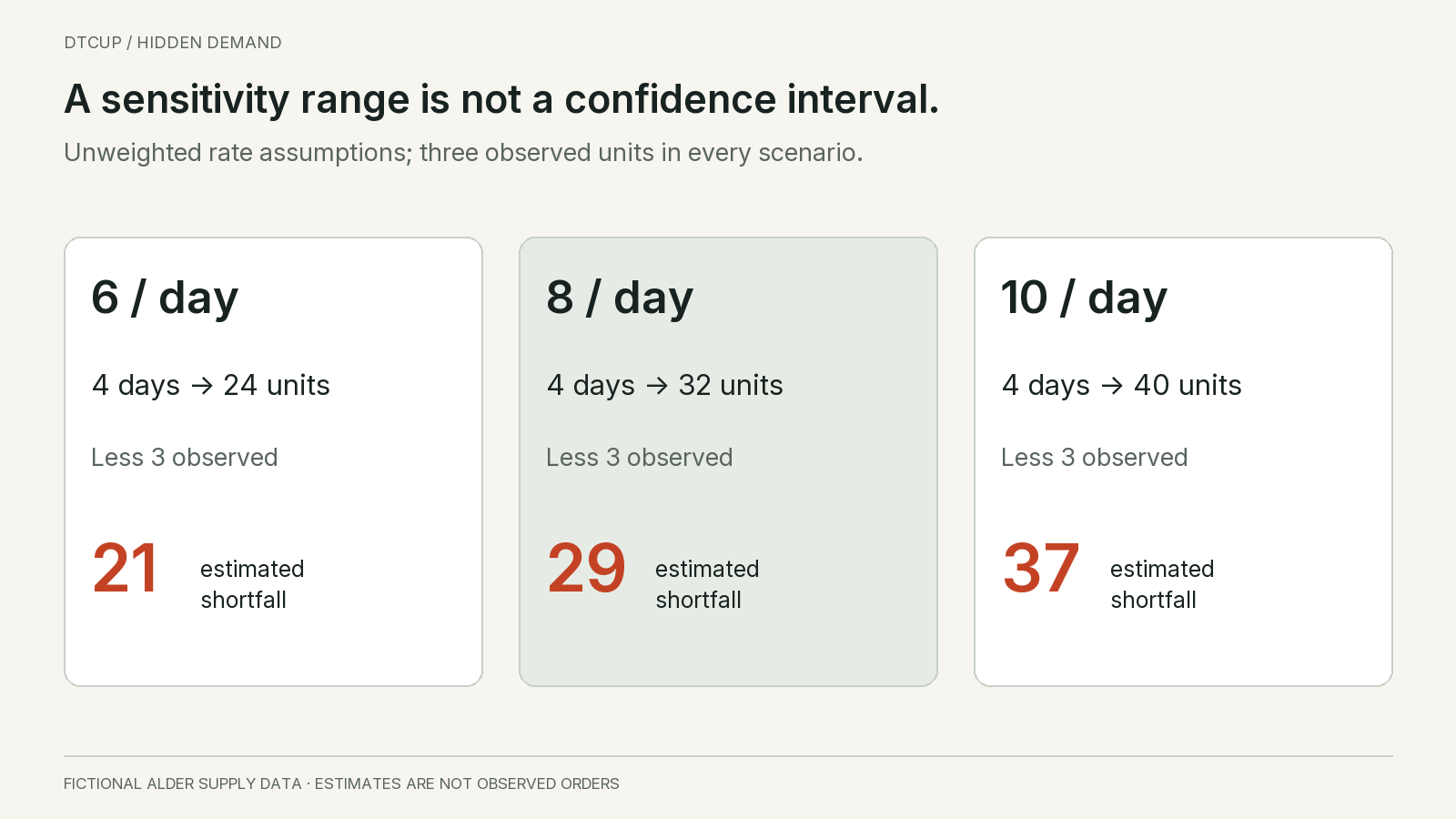
When the evidence is limited, I would show a small sensitivity table. For illustration, assume six, eight or ten units of unconstrained demand per affected day. Across four days, those rates imply 24, 32 or 40 units. Subtract the three observed units and the estimated shortfalls are 21, 29 or 37.
These are unweighted scenarios. They are not a 95 percent prediction interval, and the middle value is not automatically the most likely outcome. The range was selected to examine how a plausible rate assumption changes the result. If the business wants probabilistic coverage, it needs a validated model and a defensible method for estimating that uncertainty.
Use the scenarios to ask whether the decision changes. If every plausible case says a supplier shipment arrives too late for next week’s need, arguing over 27 versus 29 missing units may be less useful than addressing the timing problem. If the purchase decision changes sharply between 21 and 37, the team should seek better evidence or a more flexible commitment.
Show which assumptions drive the width. Perhaps traffic was stable but the stockout timing is uncertain. Perhaps timing is well recorded but a promotion changed customer interest. Those are different evidence gaps. A single wide range without an explanation can be as unhelpful as a single exact number.
Keep an estimate of zero available as a logical possibility when the evidence genuinely supports it. A stockout does not guarantee that every unavailable hour contained a willing buyer. But do not choose zero merely because no sale was recorded. The relevant question is what comparable evidence suggests about demand under availability, not whether the constrained transaction log is empty.
Likewise, avoid an unlimited upper scenario based on wishful thinking. A waitlist, high traffic or strong historical day can suggest interest, but each has conversion and comparability limits. A scenario should have a stated rationale and a decision use. It should not become a vehicle for whichever team wants a larger purchase order.
Preserve the version of the estimate used for each decision. Later information can improve understanding, but rewriting the old scenario without a record makes it impossible to evaluate the original judgment. Keep the assumptions, evidence date and chosen action together. That helps distinguish a reasonable decision under uncertainty from a calculation error or an ignored warning.
6. Separate focal-SKU demand from demand the business truly lost
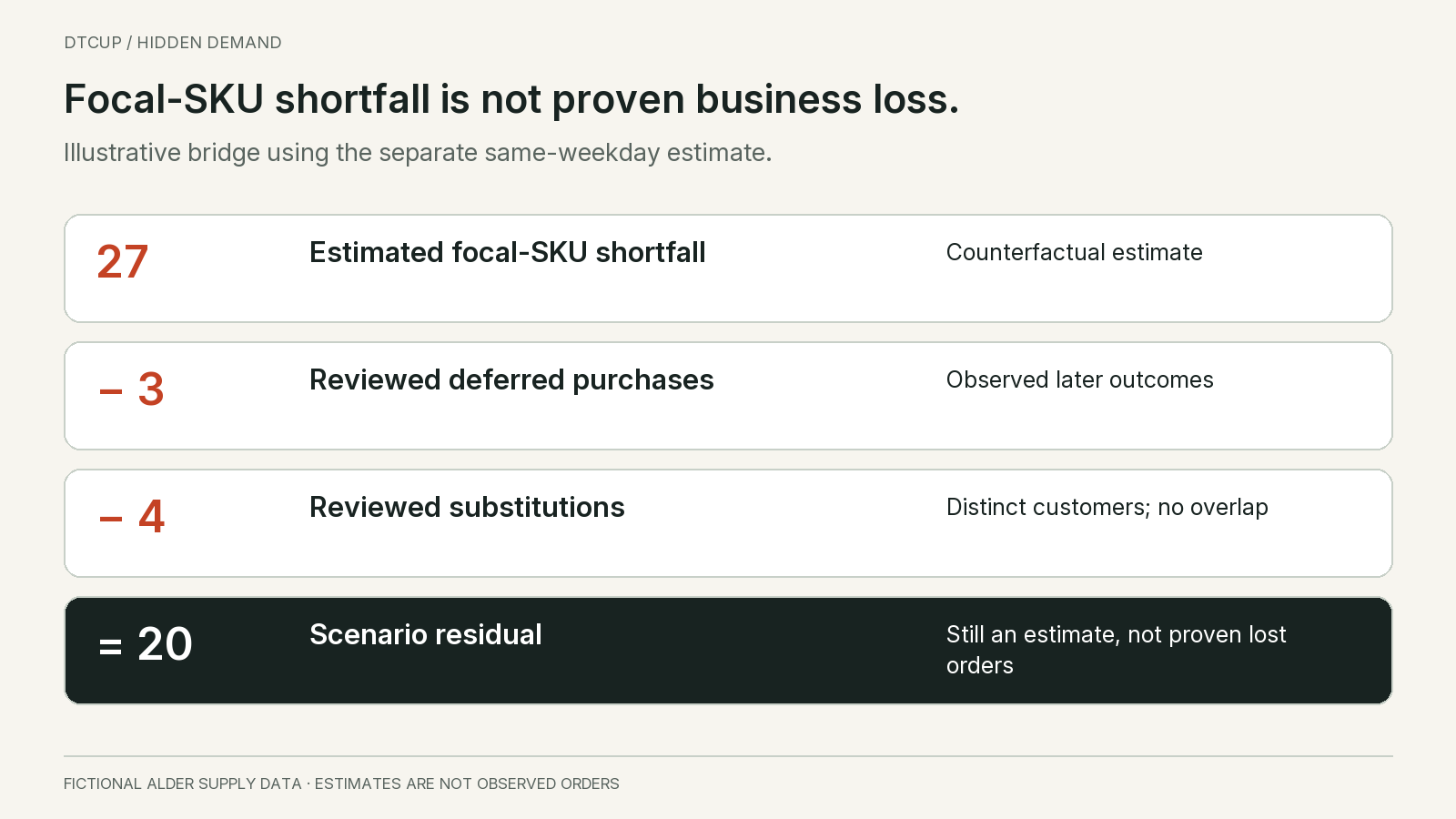
Suppose the comparison-day method suggests a 27-unit shortfall for the charcoal tray. The team later finds three customers who explicitly said they waited and then purchased that tray after replenishment. It also identifies four distinct customers who explicitly chose the sage tray because charcoal was unavailable. In this fictional example, each bought one unit, the records are reviewed, and the two groups do not overlap.
Those seven observed outcomes help explain customer behavior, but they do not validate the 27-unit estimate. The estimate concerns unobserved demand under a hypothetical availability condition. The customer records concern actual later or alternative purchases. Keep those evidence types separate, even when combining them in an illustrative bridge.
Under the assumption that all seven belong within the estimated focal-SKU shortfall, subtracting three deferred purchases and four substitutions leaves 20 units unexplained. Call that the residual in this scenario, not 20 proven lost orders. The original estimate may be wrong, other customers may have returned later, and some apparent interest may never have become a purchase under full availability.
Substitution matters differently for different decisions. The charcoal tray still experienced suppressed demand, so its future mix forecast may need attention. But the four sage purchases did not disappear from the business’s unit sales. If both variants have the same contribution margin, the immediate financial effect differs from a customer buying from a competitor. If their margins differ, the effect differs again.
Do not assume every increase in sage sales is substitution. A campaign, seasonality or an unrelated placement could explain it. The fictional example uses reviewed customer statements to make the distinction clear, but most real businesses will have incomplete evidence. In that case, show substitution as an uncertain assumption or a separate observed signal rather than claiming a precise causal transfer.
Deferred purchases also need a time boundary. A customer who waits two days and buys after restock may represent a service delay rather than a permanently lost sale. A customer who returns six months later may have a different need. Choose a follow-up window that fits the product and state it. Do not keep expanding the window until every later purchase can be credited as recovered demand.
Maintain privacy and appropriate identity boundaries when linking behavior across contacts and orders. Aggregate planning does not justify collecting unrelated personal information or forcing an identity match from weak clues. Where individual linkage is unavailable or inappropriate, use aggregate evidence with its limitations. An honest incomplete view is better than a confident but unreliable customer history.
7. Use waitlists and site behavior as evidence, not automatic orders
A back-in-stock signup is useful evidence of interest, but it is not an order. Some people sign up more than once, some are researching, some buy elsewhere and some lose interest before replenishment. Do not add every signup to estimated demand on top of a baseline that already represents the same potential customers.
Deduplicate within the permissions and identifiers available to the business, and distinguish people from requested units. One person may want two trays, while two signups may belong to the same person using different addresses. Unless the form reliably records quantity, a signup count should not be presented as a unit count.
Track the downstream response when stock returns. How many eligible signups received the notification? How many reached the relevant product page? How many placed a qualifying order within the defined follow-up window? These are different stages. A low purchase rate could reflect weak intent, a changed price, delayed replenishment, deliverability problems or an unattractive delivery promise.
Use the observed conversion of comparable prior waitlists cautiously. A previous restock with a short delay and unchanged price may not represent a current item delayed for weeks. Segment by the conditions that materially change the decision, but avoid slicing so finely that every estimate rests on a handful of people. The goal is a useful comparison, not the largest number of dashboard filters.
Product-page views and add-to-cart attempts can reveal suppressed interest, but their meaning depends on the interface. A disabled add-to-cart button may produce no event at all. A backorder-enabled cart may accept the item without an immediate purchase. A visitor can refresh repeatedly. Confirm what each event records before treating it as a demand signal.
Search activity can be another clue. Repeated searches for the unavailable variant may support the view that interest continued. Yet search counts do not establish willingness to buy at the current price or shipping terms. Use them to challenge an assumption that demand vanished, not to convert every search into a missing order.
A useful evidence table can list each signal, its observation period, its unit, its likely overlap with other signals and its limitation. Orders are units, waitlist entries may be people, and page views are events. Keeping the units visible prevents a common mistake: adding unlike quantities together because they all appear to measure customer interest.
8. Use the estimate to improve the next decision, not to create an automatic backlog
The most dangerous operational shortcut is adding the entire estimated shortfall to the next purchase order as if every missing customer were still waiting. Some demand was substituted, some deferred, some lost and some only hypothetical. The quantity needed after replenishment depends on future demand and any confirmed open obligations, not on blindly carrying forward every estimated historical unit.
Separate the future baseline from a confirmed backlog. If Alder Supply has accepted paid backorders for twelve units, those are real obligations and should be represented once in the supply plan. If it has twenty waitlist signups, those are interest signals with uncertain conversion. If it estimates a 27-unit historical shortfall, that is neither a paid backlog nor a guarantee of a restock surge.
Check whether the forecast already includes open order demand. Some planning systems forecast new orders and add the backlog separately. Others begin from a combined demand schedule. Either design can work when defined clearly, but mixing them double-counts obligations. The same care applies to replenishment-notification campaigns that are already included in a promotion forecast.
For a simple illustration, suppose the next seven days after restock have a baseline of 56 new units, and twelve verified backorder units remain to be fulfilled. If the baseline explicitly excludes those backorders, the demand schedule begins at 68 units before other adjustments. Do not then add all 27 estimated historical shortfall units. That would assume unresolved demand persists and risks counting the same customers twice.
If the team expects a restock campaign to create additional orders, model that as a separate, explicit scenario. Specify the audience, timing, comparable response evidence and whether the effect is incremental to the baseline. A campaign sent to waiting customers may accelerate purchases that would otherwise occur later rather than create entirely new demand. The inventory timing still matters, but the interpretation should remain clear.
Connect the demand schedule to sellable stock and receipt timing. A larger order arriving in six weeks cannot serve a shortage expected in three days. The relevant action may be reallocating existing stock, revising a campaign, offering an approved substitute or changing the customer promise. An estimate becomes useful only when it informs an action that can affect the period in question.
Consider the cost of uncertainty when negotiating supply. A smaller initial commitment with a confirmed later release option may be preferable to a large irreversible order when the missing-demand estimate is fragile. But supplier flexibility must be real and documented. Do not write a split-delivery scenario as if it were available before the supplier has agreed to quantities, timing and terms.
Use the estimate to investigate structural causes too. Repeated shortages of the same variant may reflect a poor mix forecast, inaccurate stock records, long inspection delays or allocation rules that leave stock in the wrong channel. Raising the total forecast without addressing that constraint can increase inventory elsewhere while the customer-facing item remains unavailable.
9. Validate the method without pretending hidden demand became observable
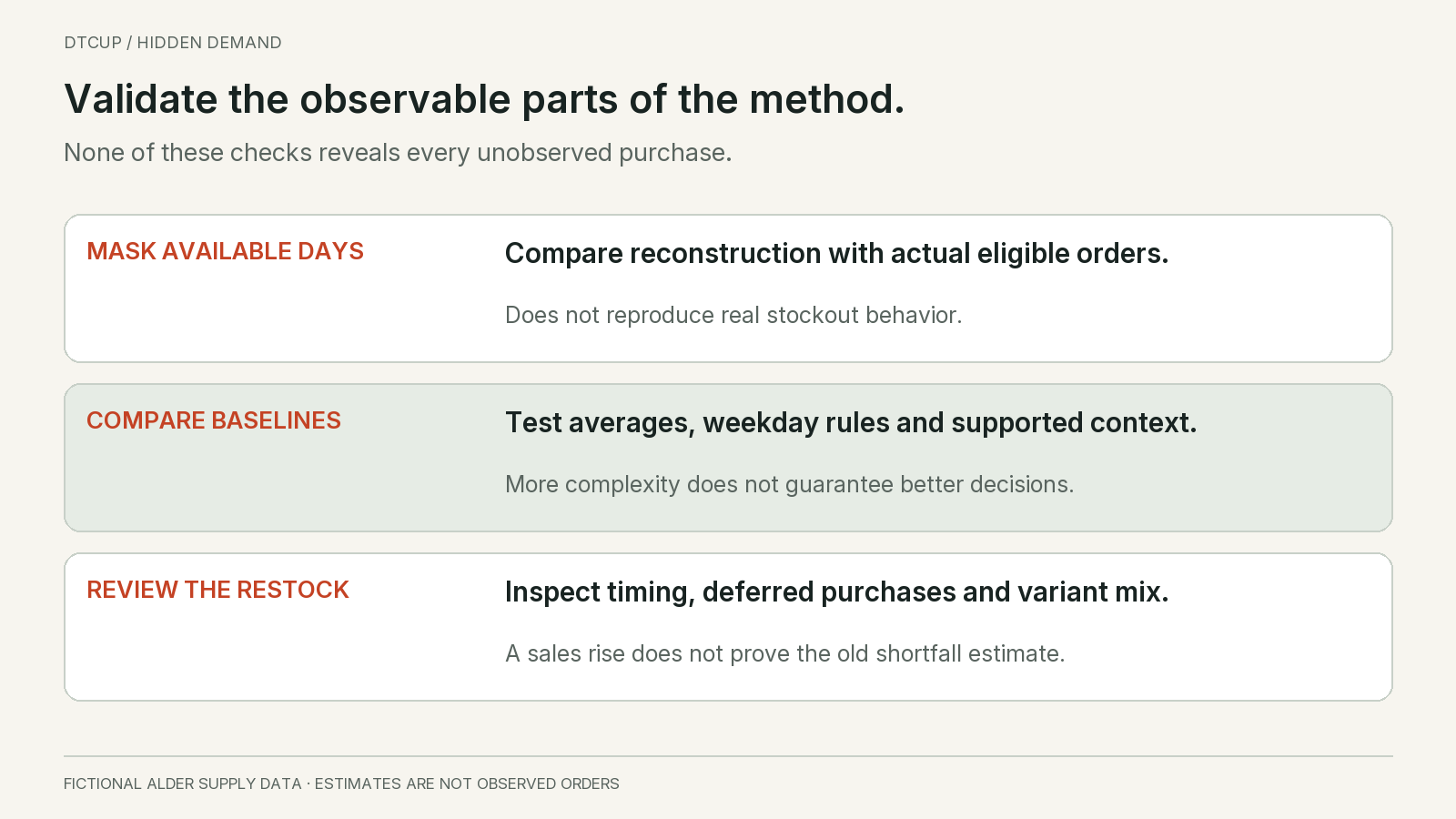
You cannot directly compare an estimated lost sale with a transaction that never occurred. That makes validation harder, but not impossible. Start by checking the method on periods where availability was verified. Hide selected observations, estimate them from information that would have been available at the time, and compare the estimate with the actual eligible orders.
This artificial masking exercise tests part of the method. It does not reproduce every consequence of a real stockout, because real stockouts can change traffic, customer behavior and substitution. State that limitation. A method that reconstructs ordinary available days well may still fail when a major campaign stops because inventory disappears.
Use time-respecting validation. Do not estimate a past day using later information that the planner would not have known if the purpose is to evaluate the original decision process. A retrospective historical reconstruction can use later evidence, but it should be labeled differently from an operational forecast. Mixing the two makes the system look more capable than it was at the decision date.
Compare simple alternatives before adding complexity. The recent available-day average, same-weekday comparison and a modest contextual model may each perform differently. Evaluate not only average error but systematic underestimation, sensitivity to promotions and the stability of the resulting supply decision. A more elaborate method is not automatically better if its assumptions are poorly supported.
Inspect the availability labels during validation. If supposedly available days contain hidden checkout failures or partial stockouts, the target itself is constrained. The model may be penalized for estimating demand above an already limited sales observation. Data-quality review and model review need to work together rather than treating the historical label as unquestionable truth.
After replenishment, compare the restock response with the scenario you documented. Did deferred customers return? Did the focal variant regain its normal share? Did a campaign create a short surge? These observations can update future assumptions, but they do not reveal every customer who left during the shortage. Avoid declaring the old lost-demand estimate proven simply because sales rose when stock returned.
Record when the method should not be used. A product discontinued for a quality concern, a broken checkout, an extreme price change or a long absence with little relevant history may fall outside the baseline’s intended scope. In those cases, use a different planning frame or an explicitly limited judgment. A reliable process includes a way to say that the available data does not support the usual calculation.
10. Turn the uncertainty into an explicit expedite decision
Consider a separate forward-looking decision at Alder Supply. The supplier can move 24 already-ordered trays onto an earlier shipment for an additional three dollars per tray. The total extra freight is therefore 72 dollars. The earlier receipt would open four additional selling days before the ordinary shipment arrives. The supplier has confirmed this option in the fictional example; it is not merely a planner’s preferred delivery date.
The historical shortfall estimates can inform the discussion, but they do not establish how many additional orders the early receipt will create. Some customers would wait for the ordinary receipt, some would buy another variant and some would not return. The relevant quantity for this commercial comparison is incremental business contribution from receiving earlier, not every unit sold during those four days.
Assume, only for this example, that each genuinely additional tray sale contributes ten dollars after the ordinary variable costs and before the extra freight. If earlier availability generates four additional sales, the contribution is 40 dollars and the result after 72 dollars of extra freight is negative 32. If it generates eight additional sales, the result is positive eight. If it generates sixteen, the result is positive 88.
The simple break-even point is 72 divided by ten, or 7.2 genuinely additional units. With whole units, at least eight are needed to exceed the extra freight under these assumptions. That is a clearer question for the team than “Do we believe the lost-sales estimate?” It asks whether enough customers are likely to be retained by the earlier arrival to justify the specific incremental cost.
This calculation is deliberately narrow. It omits customer-experience value, future repeat purchases, supplier reliability changes and other effects that might matter. It also assumes the ten-dollar contribution is appropriate and that the 72-dollar charge is the complete incremental freight cost. If extra handling, duties or other costs change with the option, include them before using the comparison.
Do not count a customer who would have bought the same tray four days later as an entirely new ten-dollar contribution without explaining the timing benefit being valued. Earlier cash receipt or better service may have value, but it is not the same as preventing a permanently lost sale. Similarly, a customer switching from an equally profitable sage tray may change the variant mix without adding ten dollars of business contribution.
Check the physical limit and the next period. The earlier shipment contains only 24 trays, so it cannot serve unlimited demand. If selling those trays early leaves another channel short, the apparent benefit may be offset elsewhere. The comparison should include the allocation consequence rather than treating stock moved from one customer group to another as newly created supply.
Use the three scenarios as a discussion aid, not as invented probabilities. The team might have credible evidence that several paid orders will otherwise be canceled, which strengthens the early-receipt case. It might instead have only anonymous page views and an uncertain arrival promise, which weakens it. Document the evidence for the incremental-sales assumption and the supplier’s timing commitment.
Arrival uncertainty can overturn the result. An expedited shipment that is only likely to arrive one day earlier than the ordinary shipment may provide far less benefit than a guaranteed four-day improvement. Do not multiply the best-case selling window by a confident demand rate while ignoring the uncertainty in receipt timing. Consider the feasible arrival scenarios together with demand.
If the decision remains sensitive, seek a smaller or more reversible option. Perhaps the supplier can expedite fewer units, or the business can serve confirmed backorders first while communicating the ordinary receipt to other customers. Those possibilities need confirmation and may have different per-unit charges. The right next step is to investigate a feasible option, not to invent flexibility in the spreadsheet.
Afterward, compare what happened with the decision record. Record the actual extra freight, arrival date, allocation and observed orders, along with what can and cannot be concluded about incrementality. Do not label every early-period order a rescued sale. Even an imperfect review can improve the next decision if it preserves the distinction between transactions observed and customer behavior inferred.
11. Keep a short decision record that prevents the same argument next month
For each material shortage, preserve the focal SKU and channel, the constrained interval, the availability evidence, the original eligible orders, the comparison rule and the scenario results. Add the supply decision and the next review date. A concise record is more useful than a large analysis file whose assumptions are remembered only by its author.
Show observations and estimates with different labels in the planning view. Do not use a solid historical sales line for imputed demand without a clear distinction. A future reviewer may otherwise treat the reconstructed series as actual transactions and use it in another model, compounding the original assumptions.
Assign responsibility for the availability data. Marketing may know when ads stopped, operations may know when stock became sellable, and the website team may know when the purchase control changed. Planning needs those events connected, but no single team should be expected to infer all of them from an order export.
Review the estimate when material evidence arrives. A corrected stockout timestamp, confirmed supplier receipt or verified backorder count can change the decision. Do not revise the estimate every hour merely because another page view appears. Choose update triggers that correspond to a meaningful change in the demand or supply picture.
Keep commercial interpretation separate from financial reporting. Estimated unmet units can inform a contribution scenario, but they are not recognized revenue or a booked loss. If a decision needs a money estimate, define price, variable costs, substitution and timing assumptions explicitly. Do not multiply a speculative unit shortfall by retail price and present the result as a verified financial loss.
The practical aim is to stop availability failures from disguising themselves as weak demand. Preserve what happened, estimate what might have happened with visible assumptions, and use the difference to make a better supply decision. The estimate should make uncertainty easier to manage, not make it disappear from the report.
Sources
Still have a question?Ask the DTCUP Community ↗