
Safety Stock Is a Service Decision, Not a Universal Percentage
A larger buffer can reduce shortages while tying up cash. Compare service measures, replenishment horizons and realistic demand scenarios before turning a safety-stock formula into a buying rule.

7 years of experience building and operating brand websites, specializing in website development, paid advertising and SEO. Built a brand website from launch to US$10 million in annual sales.
The Short Answer
Define the customer service outcome first, then match the buffer to the replenishment horizon, demand uncertainty and supply behavior. Test the complete purchasing policy against shortages, inventory and cash rather than treating one percentage or formula as a guarantee.
Key takeaways
- Cycle service and unit fill rate answer different questions.
- A reorder trigger is not the same as a periodic order-up-to target.
- Simple formulas depend on assumptions about demand and lead time.
- Joint demand and supply stress deserves separate scenarios.
- Average service can hide failures in important low-volume items.
- Record the buffer, owner, assumptions and next review in a policy card.

“Keep an extra twenty percent” is an easy safety-stock rule to communicate. It is much harder to explain what that extra inventory protects. Twenty percent of which demand, over which period, against which uncertainty, and with what promise to the customer?
A buffer should be the consequence of a service decision and a replenishment process. It should not be an unexplained number added to every purchase order. Otherwise, the team can hold too much of predictable products while still running out of items whose supply or demand is genuinely uncertain.
The useful starting question is: “What kind of shortage are we trying to avoid, and how much uncertainty must the inventory absorb before we can respond?” That question connects the customer promise, demand, supplier timing, buying cadence and cash. The formula comes afterward.
This guide uses Solace Home, a fictional home-accessory business, to build a safety-stock decision. All quantities, lead times, cost assumptions and scenario results are constructed. They are not customer results or suggested targets for every business. The calculations are deliberately transparent so you can see which assumptions would need replacing.
I would use a statistical calculation as a candidate policy, then test how that policy behaves in the actual operation. The final decision should explain both the desired service and the inventory burden. A precise spreadsheet answer is not enough if the warehouse, supplier or buyer operates differently from the model.
First, define what “good service” means
A team can agree on ninety-five percent service while disagreeing completely about what that number means. One person may mean avoiding a stockout in ninety-five percent of replenishment cycles. Another may mean supplying ninety-five percent of requested units immediately. Another may mean shipping ninety-five percent of complete orders on time.
Those are different measures. Cycle service describes the frequency of cycles without a shortage. Unit fill rate describes the share of requested units supplied under the defined immediate-availability rule. Complete-order performance also depends on whether every required line is available and on the shipping process.
NC State’s inventory tutorial distinguishes cycle service from demand fill rate. The practical lesson is to name the measure and its denominator before choosing a target. A percentage without that definition is not a usable purchasing instruction.
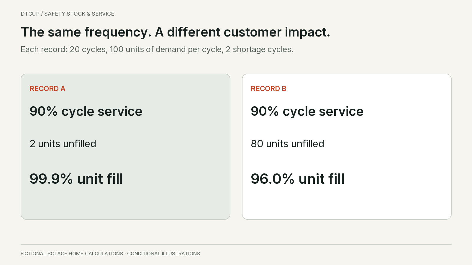
Consider two constructed operating records. Each contains twenty cycles with one hundred units of demand per cycle, or two thousand units in total. In both records, eighteen cycles have no shortage and two have a shortage. Both therefore show ninety percent observed cycle service.
In the first record, each shortage affects one unit. Two units out of two thousand are not filled immediately, giving a unit fill rate of 99.9 percent. In the second, each shortage affects forty units. Eighty units are not filled immediately, giving a fill rate of ninety-six percent.
The same cycle-service result can therefore hide very different customer impact. This does not make cycle service useless. It means that the frequency and size of shortages answer different questions. Choose the primary measure for the decision and retain useful secondary measures rather than blending them into one ambiguous score.
Also define whether unfilled demand waits or disappears. A backorder may be delivered later; a lost sale may never become an order. Immediate fill, eventual fulfillment and revenue recognized this month will then differ. Preserve those meanings when evaluating the policy.
Find the period during which the business cannot fully respond
Safety stock protects against uncertainty during an exposure period. The supplier’s transit time is only part of that period. Order approval, production, booking, transport, customs, receiving and inspection may all matter before units become sellable.
Choose a start and end event. For Solace’s example, lead time begins when a valid replenishment order is released and ends when the units are available for sale at the intended location. A supplier’s dispatch date is not the same as that end event.
Then identify how often the buyer can act. A system that continuously reviews inventory can place an order when a trigger is reached. A buyer who reviews the item only once a week may wait several days before placing the next order. That waiting period changes the exposure.
In a simple periodic review arrangement, the protection interval includes the review interval plus replenishment lead time. Rossetti’s inventory systems chapter explains the distinction between continuous and periodic review. The operating implication is simple: a weekly buying process should not quietly use a calculation that assumes immediate response.
Do not add every named delay mechanically. Some activities overlap, and some are already included in the measured end-to-end lead time. Map the actual sequence and measure the elapsed time between the agreed endpoints. Double-counting the same delay inflates the buffer; omitting receiving time understates it.
Separate routine variation from exceptional disruption. A supplier varying between eight and eleven days is different from a port closure that makes the route unavailable. Both matter, but an ordinary statistical buffer may not be the best or only response to the second situation.
Write the protection horizon beside the safety-stock number. “Thirty units for demand variation over nine days under continuous review” is much more informative than “safety stock: thirty.” The first can be challenged when the process changes; the second tends to survive long after its assumptions are forgotten.
A simple calculation, with its assumptions left visible
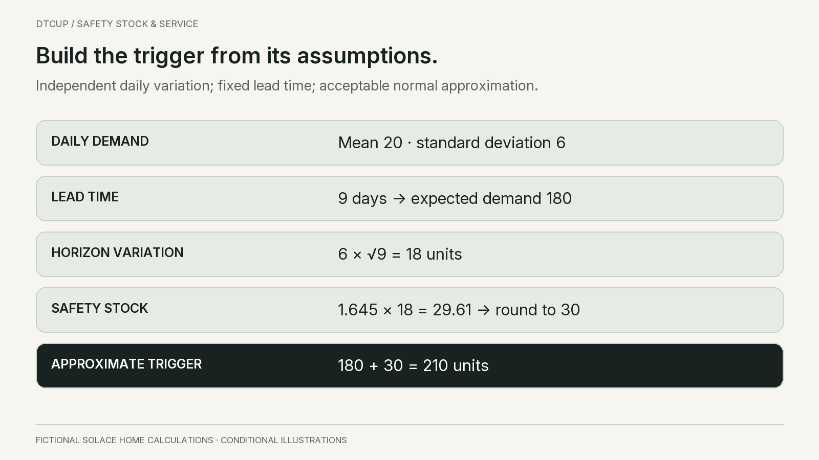
Solace begins with a regularly selling item. Assume average daily demand is twenty units and the standard deviation of daily demand is six units. Lead time is fixed at nine days. Daily demand fluctuations are assumed independent, and a normal approximation for total lead-time demand is treated as acceptable for this illustration.
Expected demand over nine days is twenty multiplied by nine, or one hundred eighty units. Under the independence assumption, the standard deviation over that horizon is six multiplied by the square root of nine, or eighteen units. Standard deviations do not simply add across independent days.
For an illustrative ninety-five percent cycle-service target under the normal approximation, use a one-sided standard-normal factor of approximately 1.645. Multiplying 1.645 by eighteen gives 29.61 units of safety stock. Rounding the buffer upward gives thirty units, and the corresponding approximate reorder point is two hundred ten units.
The familiar relationship is reorder point equals expected lead-time demand plus safety stock. Peter King’s safety-stock article, hosted by MIT presents this style of variability-based calculation. Here, the numbers are original teaching assumptions, and the result is conditional on them.
Two cautions are essential. First, the ninety-five percent refers to the chosen model’s cycle-service target, not a guarantee that ninety-five percent of all customer orders will arrive on time. Second, rounding and a normal approximation do not turn a discrete, changing real operation into an exact theoretical system.
The calculation is also not a purchase quantity. Under a continuous-review policy, the reorder point is compared with the defined inventory position, and the ordering rule determines how much to order. Buying two hundred ten units every time because the reorder point is two hundred ten would confuse the trigger with the order size.
Inventory position commonly includes on-hand stock plus outstanding supply minus backorders, with operational adjustments defined carefully. Do not subtract the same reservation twice or count unsellable stock as freely available. Timing still matters: supply arriving too late cannot prevent a shortage before its arrival.
That last point is why a dated inventory projection remains useful even when the reorder calculation is correct. A scalar position summarizes a policy state; it does not show every future day when stock may become unavailable.
What changes when purchasing happens weekly
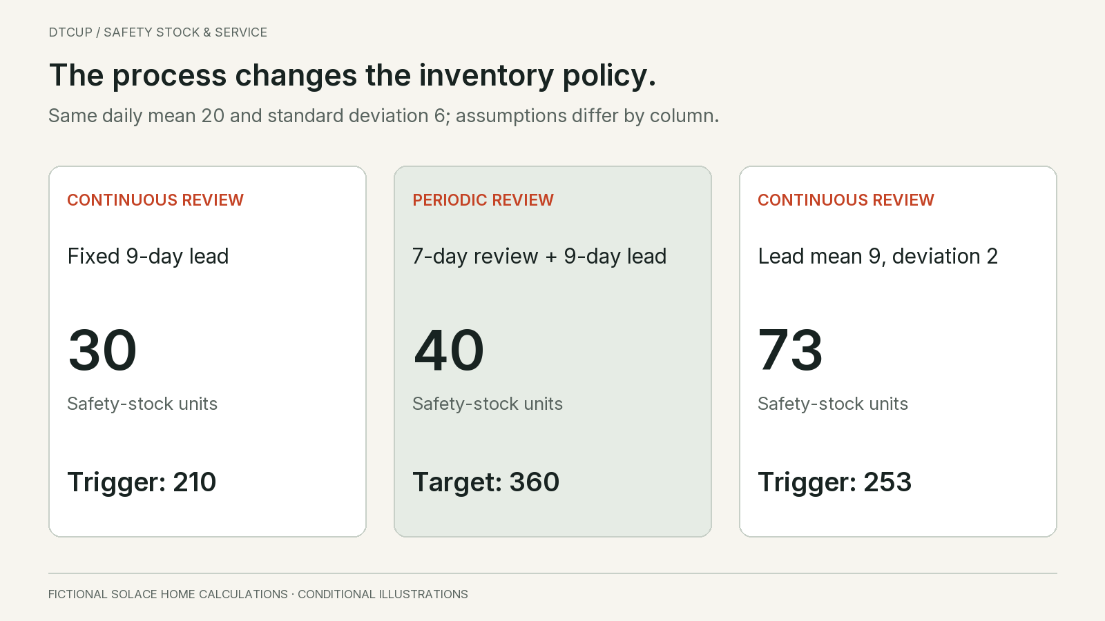
Now keep the same demand assumptions and nine-day lead time, but let Solace review this item every seven days. The simple protection horizon becomes sixteen days. Expected demand over that horizon is three hundred twenty units.
With independent daily variation, the horizon standard deviation is six times the square root of sixteen, or twenty-four units. Multiplying by 1.645 gives 39.48 units. Rounding upward produces forty units of safety stock and an illustrative order-up-to target of three hundred sixty units.
That target is not directly comparable with the earlier two-hundred-ten-unit reorder trigger as if both were quantities to buy. They belong to different control rules. One says when to replenish under continuous review; the other says what position to restore at a scheduled review under the stated periodic model.
At the weekly review, suppose the defined inventory position is two hundred forty units. Before pack-size or other adjustments, the proposed replenishment is three hundred sixty minus two hundred forty, or one hundred twenty units. The target tells the buyer where to restore the position, not that every order must contain three hundred sixty units.
If the supplier accepts only full cartons, the feasible quantity may differ. If there is a firm order consuming part of the forecast, the planning logic must avoid double-counting it. If an outstanding receipt is late, the date projection may reveal a shortage even though the inventory-position arithmetic appears adequate.
Changing the review cadence can therefore be an inventory decision. More frequent reliable review may reduce exposure, but it can increase ordering effort or transport cost. The benefit should be compared with the complete operating cost, not celebrated as free inventory reduction.
The key is consistency. If the spreadsheet assumes daily action but the purchasing meeting happens on Mondays, the model and the process disagree. Fix that mismatch before debating whether the statistical factor should be slightly higher or lower.
Lead-time uncertainty can dominate demand uncertainty
Return to continuous review and keep the daily demand mean at twenty and standard deviation at six. Now suppose lead time averages nine days with a standard deviation of two days. For this example, daily demand is independent across days and independent of the random lead time.
Under that random-sum setup, lead-time demand variance is the average lead time multiplied by daily demand variance, plus the square of average daily demand multiplied by lead-time variance. Numerically, that is nine times thirty-six plus four hundred times four, or one thousand nine hundred twenty-four.
The square root is approximately 43.86 units. Using the same 1.645 factor gives approximately 72.16 units of safety stock, rounded up to seventy-three. Expected lead-time demand remains one hundred eighty units, producing an approximate reorder point of two hundred fifty-three units.
The buffer is now much larger than thirty even though average daily demand and average lead time did not change. The extra uncertainty comes from the replenishment timing. A demand-only calculation would miss that part of the problem.
This formula has conditions. If demand and lead time move together, or daily demand has important serial correlation, the simple independence calculation may be unsuitable. A promotional peak that increases demand while slowing supplier processing is exactly the kind of situation that deserves a joint scenario rather than a casual independence assumption.
Also examine how lead time was measured. Completed orders alone can underrepresent the longest outstanding delays. A receipt may be split across several deliveries. A supplier’s promised date and the actual sellable-receipt date are different data fields. Preserve those distinctions before estimating variation.
For Solace, the decision is not automatically “buy forty-three more units forever.” The comparison suggests investigating supply reliability. If a receiving bottleneck or inconsistent booking process creates avoidable delay, improving it may reduce uncertainty more effectively than financing a permanent buffer.
At an assumed twenty dollars per unit, an additional forty-three units represent eight hundred sixty dollars of inventory investment. That is cash tied up in stock, not an immediate expense of the same amount. If a hypothetical annual carrying charge is twenty-five percent, the associated annual carrying-cost estimate is two hundred fifteen dollars, before other relevant consequences. Use the business’s own cost basis.
Use uncertainty in the right quantity
A historic standard deviation can combine predictable patterns with genuine uncertainty. If demand rises every weekend, treating the entire weekend pattern as random noise may exaggerate the uncertainty that remains after forecasting. If a promotion is planned, its expected effect belongs in the demand plan rather than being hidden entirely in safety stock.
Where a forecast is used, examine errors over the relevant replenishment horizon. Compare what was predicted at the decision date with what subsequently occurred over that horizon. This is different from calculating the variation of all daily sales around one long-term average.
Preserve the information available at the time. A forecast reconstructed after seeing the outcome can look much more accurate than the one the buyer actually used. The forecast backtesting guide explains how to evaluate the decision without leaking future information into the past.
Correct persistent bias before treating it as random uncertainty. If the forecast repeatedly understates normal demand, an ever-larger buffer may conceal the problem. The mean demand plan and the uncertainty allowance have different jobs. Both may need attention, but they should not become an unexplained combined number.
Watch for constrained observations. Sales recorded during a stockout may understate the demand the inventory policy should have served. Missing imports are not zero demand. The stockout-demand guide describes how to preserve that uncertainty instead of feeding suppressed sales into a confident buffer calculation.
For intermittent items, a normal approximation may be a poor description of many zero periods followed by occasional batches. A fractional mean does not describe the next request. Use an appropriate demand distribution or scenario approach and examine the resulting service policy, as discussed in the slow-seller forecasting guide.
Finally, be honest about sample size. A few replenishment cycles provide limited evidence about a rare tail. The largest observed demand is not a proven worst case, and an estimated high percentile from a tiny sample should not be presented as a dependable guarantee. Record the uncertainty and plan how the estimate will improve.
Compare candidate stock levels before choosing one
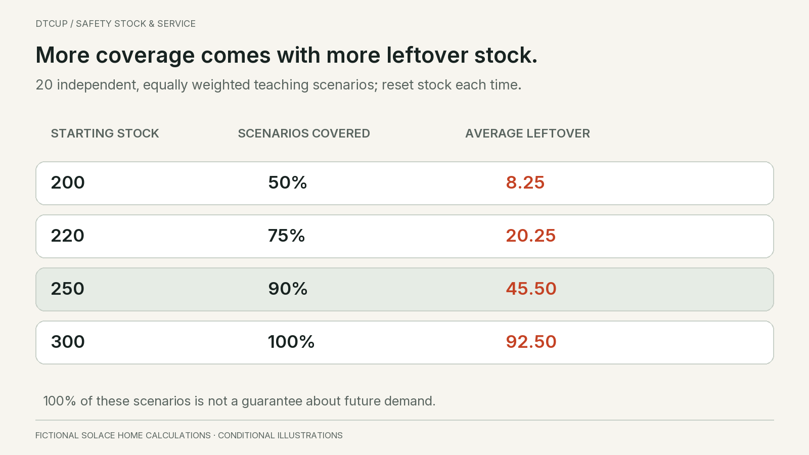
A scenario table can make the tradeoff visible without pretending that one formula settles the decision. For a separate teaching exercise, consider twenty possible exposure periods with total demand of 160, 170, 175, 180, 180, 185, 190, 195, 200, 200, 205, 210, 210, 215, 220, 225, 230, 240, 260 and 300 units.
These scenarios are constructed and equally weighted for the exercise. Each starts fresh with the candidate stock level and receives no replenishment during its exposure period. Leftover stock is not carried into the next scenario. This is a one-period exposure comparison, not a simulation of a continuous replenishment policy.
Total demand across the twenty scenarios is four thousand one hundred fifty units. For each candidate, calculate unmet units as the positive difference between demand and starting stock. Calculate leftover units as the positive difference between starting stock and demand. Count a scenario as fully covered only when demand does not exceed stock.
| Starting stock | Fully covered scenarios | Unmet units across scenarios | Units filled across scenarios | Average leftover units |
|---|---|---|---|---|
| 200 | 10 of 20, or 50% | 315 | 92.4% | 8.25 |
| 220 | 15 of 20, or 75% | 155 | 96.3% | 20.25 |
| 250 | 18 of 20, or 90% | 60 | 98.6% | 45.50 |
| 300 | 20 of 20, or 100% | 0 | 100% | 92.50 |
The table shows why the business must name the service objective. Two hundred fifty units cover eighteen scenarios completely and fill approximately 98.6 percent of total scenario demand. Those are different descriptions of the same candidate. Selecting it because it “achieves about ninety-nine percent service” would omit a meaningful distinction.
Moving from two hundred fifty to three hundred units eliminates the sixty unmet units in this constructed set. It also increases average leftover stock by forty-seven units. Whether that is worthwhile depends on the consequence of shortages, the value of leftover stock and the actual probability of comparable outcomes.
The table does not establish a real-world optimum. Equal scenario weights are an assumption. The scenarios may omit disruption or obsolescence. Inventory cost depends on time and replenishment behavior, not only end-of-period leftovers. Use the table to structure the decision, then test the actual policy with appropriate data and constraints.
Most importantly, full coverage of these twenty scenarios is not a promise of no future stockouts. A sample maximum is not a physical limit on demand. A planner who selects three hundred should still document what happens if demand exceeds it or supply arrives later than the scenario assumed.
Stress the conditions that can fail together
Demand and supply do not always vary independently. A seasonal peak can increase orders while suppliers and carriers become busier. A promotion may coincide with a receiving backlog. A weather event can affect both demand for an item and the route used to replenish it.
For a simple stress case, suppose daily demand becomes twenty-eight units while the sellable-receipt lead time becomes fourteen days. The exposure demand is three hundred ninety-two units. That is two hundred twelve units above the earlier baseline of one hundred eighty.
This is not a probabilistic forecast and it does not imply an exact shortage of two hundred twelve units. Actual stock, outstanding receipts and timing would determine the shortage. The calculation asks whether the operation has a credible response to a joint change much larger than ordinary independent fluctuations.
Possible responses include earlier ordering, a qualified alternative source, a transport option, allocation rules, a revised customer promise or a temporary promotion limit. Each has cost and feasibility constraints. Some may be more useful than carrying enough stock to cover every imaginable disruption throughout the year.
Do not assume a backup supplier is available because its name appears in a spreadsheet. Check qualification, capacity, lead time, compatibility and the actual ability to place an order. A contingency that cannot be activated within the exposure period is not an immediate substitute for inventory.
Keep ordinary safety stock and contingency planning distinct in the decision record. Ordinary buffers handle the variation the policy is designed around. Contingencies handle named situations outside that routine range. Combining both into one inflated percentage makes it difficult to know when inventory can be reduced or when a contingency should activate.
Review the stress cases with the people who operate the process. The supplier manager may know about a shutdown; the warehouse may know receiving capacity is constrained; marketing may know a launch date is fixed. A statistical model cannot incorporate information the organization never supplies.
Set different service policies for different customer consequences
Not every item deserves the same service target. A replacement component needed to make an existing product usable has a different role from an optional decorative accessory. A short-lived seasonal design has different leftover risk from a stable replenishment item. Revenue rank alone does not capture those differences.
Start with the customer consequence of unavailability. Can the customer reasonably substitute another item? Can they wait? Does the missing component prevent use of a larger purchase? Would a shortage affect a contractual or established service commitment? These questions help define the policy before assigning a percentage.
Then consider recovery. An item with a dependable short replenishment route may need a different buffer from one with a long, uncertain route. The same demand variability can produce very different exposure when response time differs.
Consider the inventory downside too. Perishability, product revisions, fashion risk, storage requirements and cash limits can make excess units costly. A service decision should acknowledge those costs rather than treating the highest target as automatically superior.
For Solace, the review might create three operating groups: essential service items with a defined availability commitment; stable core sellers with a balanced replenishment policy; and limited-life products with an explicit end-of-season plan. These are illustrative groups, not a universal classification. The business should choose categories that lead to different useful actions.
Do not let segmentation become an opaque label. Each group needs a service measure, a target rationale, a replenishment approach and an exception owner. If two groups receive identical treatment despite different names, the classification is adding administrative work without improving decisions.
Review items that cross boundaries. A slow accessory may become essential when bundled with a core product. A once-stable item may approach discontinuation. Policy should follow the item’s current role, not remain attached to a historic sales ranking.
Check the stock state before changing the buffer
Portfolio reporting needs the same care as item-level planning. Suppose a fast seller has ninety-nine percent immediate unit fill while a small service part is unavailable for long periods. A unit-weighted total can still look excellent because the fast seller dominates the denominator. That does not mean the service-part promise is being met.
Keep a portfolio measure for overall volume, but also inspect the items whose shortage has a disproportionate consequence. This is not an argument for giving every small item the highest target. It is an argument for making the customer role visible instead of allowing a large denominator to hide it.
For example, one fictional item fills nine hundred ninety of one thousand requested units, while another fills fifty of one hundred. Their individual fill rates are ninety-nine and fifty percent. The combined unit fill rate is one thousand forty divided by one thousand one hundred, approximately 94.5 percent. Averaging the two percentages instead gives 74.5 percent, which answers a different, equally weighted item question. Neither calculation should be presented without its weighting. A buyer reviewing the second item’s service problem needs to see its fifty unfilled units even when the portfolio dashboard emphasizes the larger item’s volume.
A complete-order promise adds another complication. If an order requires several components, each component’s availability does not directly equal the order’s availability. The relationship depends on which items are ordered together and whether shortages occur together. Do not multiply or average item service percentages casually and label the result an order-service guarantee.
Pooling inventory across locations can sometimes reduce the total buffer needed, but only when stock can actually reach the customer in time. A central spare unit is not equivalent to a local unit if transfer takes longer than the promised response. Shared disruption can also limit the diversification benefit that a simple pooling argument assumes.
For Solace, this leads to a practical review question: which customer commitments rely on this stock location, and what alternatives remain when it is empty? The answer may support a local buffer, a central reserve or a different promise. The location policy should follow that operating reality.
Some apparent safety-stock failures are inventory-record failures. The system may count damaged, quarantined or reserved goods as available. A purchase order may remain open after cancellation. A receipt may be recorded before the warehouse can pick the units. Increasing the buffer can conceal these errors without resolving them.
Define sellable on-hand stock, commitments and incoming supply clearly. Reconcile source identifiers so the same receipt is not counted twice through two integrations. Preserve location because stock in another warehouse may not be available within the customer promise.
Keep units consistent. A supplier carton, a selling kit and an individual component are not interchangeable quantities. If one kit consumes two components, the demand and supply calculation must use the same planning unit. A perfectly calculated buffer in the wrong unit is still wrong.
Record the date of each incoming quantity and the confidence attached to that date. An overdue purchase order is not equivalent to a confirmed receipt tomorrow. A broad inventory-position measure may be useful for the policy, but the buyer still needs a timeline of when units become usable.
Check whether known orders have already been included in the forecast. Adding all customer commitments on top of a forecast that already expects them can double-count demand. Removing all commitments without understanding forecast consumption can create the opposite error. The rule should be explicit and consistent.
These checks should happen before escalating the service target. Otherwise, the team may approve more inventory to compensate for inaccurate availability, then discover the surplus only after the records are corrected. Fix the state first, rerun the candidate policy and explain any remaining uncertainty.
Validate the policy through the events it would have faced
A candidate safety-stock level should be tested with the full replenishment rule. Include the review cadence, order quantity or order-up-to logic, pack sizes, supplier timing, receipts and demand treatment. A buffer alone cannot describe the behavior of an inventory system.
Use a walk-forward review where possible. At each historical decision point, use only information available then. Place the hypothetical order under the candidate rule, let the subsequent demand and receipts occur, and record service and inventory outcomes. Do not reset the stock to a convenient starting level every week unless that reset is explicitly part of a separate exposure exercise.
Keep the baseline policy in the comparison. A more complex method should improve a relevant outcome enough to justify its maintenance burden. Sometimes correcting a lead-time field or reviewing more consistently matters more than changing the statistical model.
Measure shortage frequency, unfilled units, duration of unavailability, average inventory and aged inventory as appropriate. Add expedites and other recovery costs where they are reliably observed. Do not choose a candidate solely because one error metric improved.
Inspect the difficult periods individually. A policy may perform well on average while failing during the one launch that matters most. Conversely, a policy that covers every extreme event may leave unacceptable surplus during ordinary trading. The review should make that tradeoff visible.
Distinguish simulated outcomes from actual results after release. A backtest is evidence about how a defined policy would have behaved under the supplied history and assumptions. It is not proof of future service. A live review should compare actual decisions and outcomes with the policy record, including overrides.
If the evidence is too thin, reduce the confidence of the conclusion. Use a conservative, bounded policy with explicit review triggers rather than reporting a precise high-percentile guarantee. The point is to make a better decision under uncertainty, not to eliminate uncertainty from the presentation.
Give the buyer a policy card they can operate
Before handing over the card, check that the business has not layered several allowances for the same risk. A planner might increase the forecast for a promotion, add a promotion buffer, accept a supplier’s extra quantity and then apply the standard safety-stock percentage. Each step can sound reasonable in isolation while the combined purchase protects repeatedly against the same expected demand.
Ask each adjustment to name its purpose. The forecast should include the expected demand pattern. Safety stock should cover the uncertainty defined by the policy. A carton adjustment reflects a purchasing constraint. A strategic reserve may cover a named disruption or service commitment. These quantities can coexist, but they should not all be described as ordinary safety stock.
Consider a simple illustrative purchase worksheet with expected horizon demand of three hundred units. A planner adds sixty units because a campaign is expected to increase demand. Another person adds a twenty-percent campaign allowance to the new total, creating seventy-two more units. If both adjustments represent the same expected campaign effect, the worksheet has counted it twice. If the second protects a separately justified uncertainty, document that evidence rather than relying on the label.
Round only after the unrounded recommendation and its components are visible. Suppose an otherwise justified order is one hundred twenty-three units and the carton size is twenty-four. Rounding to a feasible one hundred forty-four units adds twenty-one units because of packaging, not because demand became less predictable. Keeping that distinction helps the buyer discuss smaller packs or mixed cartons with the supplier.
Also decide when an override expires. A temporary reserve for a launch should not remain after the launch merely because nobody removed it. A supplier-delay adjustment should be reviewed when the route recovers. An exception without a date or trigger can become a permanent inventory policy by accident.
These details are where an analytically sound recommendation becomes a maintainable operating process. They let the next buyer reconstruct why the quantity exists and remove an allowance when its reason no longer applies. Without that record, inventory tends to accumulate through individually cautious decisions that nobody evaluates together.
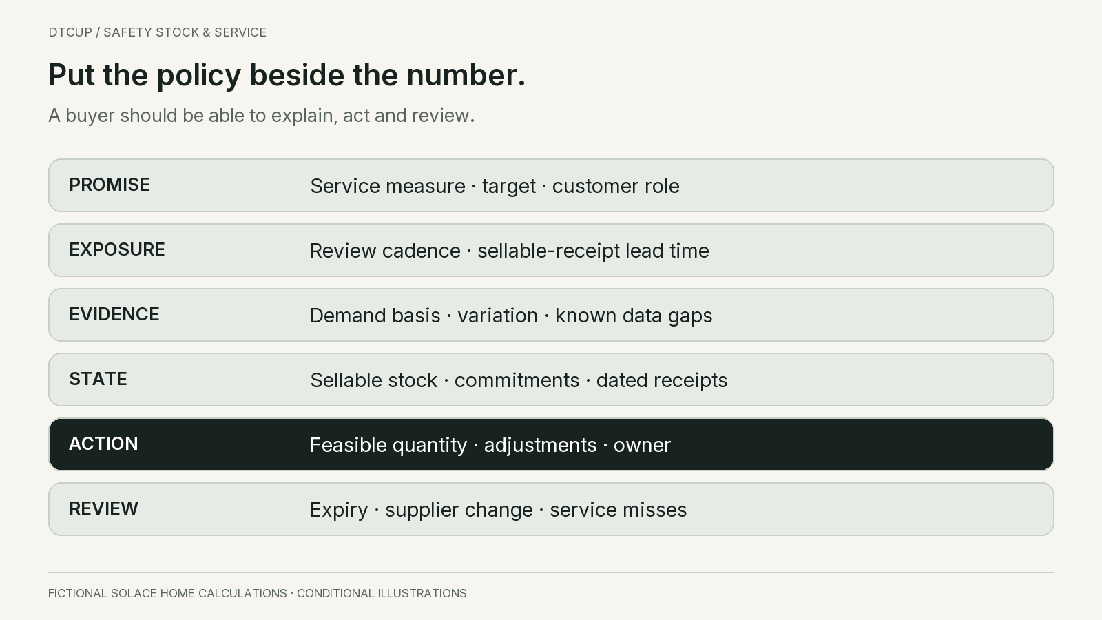
The final output should fit into a practical review. Start with item and location, the planning unit and the service role. State the primary service measure and target, then the protection horizon and the replenishment rule. These fields explain what the number is meant to do.
Show the demand and supply evidence with dates. Include the forecast version or observation window, the lead-time endpoints and any known gaps. A buyer should be able to see whether the recommendation is based on recent complete records or a provisional estimate.
Separate expected demand, uncertainty allowance and operational adjustments. If a minimum order or pack size changes the proposed purchase, show that adjustment rather than hiding it inside safety stock. If a manager approves an exception, record the reason and its expiry.
Show the action and the unresolved risk. “Order one hundred twenty units at this review, subject to carton rounding; verify the overdue receipt before release” is operational. “Inventory health: green” is not enough to explain a purchasing decision.
Include a review trigger. It might be a supplier lead-time change, a sustained forecast bias, a promotion, a new product revision or repeated service misses. A policy that is never revisited becomes a historical artifact rather than a control.
The card should also identify who can override the recommendation and how the override will be reviewed. Human judgment is valuable when it adds evidence the model lacks. It becomes difficult to learn from when changes are made silently and the original recommendation disappears.
Questions before approving a safety-stock change
Is a fixed percentage ever acceptable?
It can be a transparent temporary rule when data is limited, provided the team states what it is protecting, why that level was chosen and when it will be reviewed. Do not present it as a statistically calibrated service guarantee. Replace or refine it as the operating evidence improves.
Should we raise the target after every stockout?
No. First identify whether the event came from expected variation, biased demand, late supply, incorrect records or a process failure. A stockout can be consistent with a policy that deliberately accepts some risk. It can also reveal a broken assumption. The response should follow the cause rather than automatically adding units.
Can we remove safety stock if forecasting becomes more accurate?
Better forecasting may reduce demand uncertainty, but lead-time variation, execution problems and other exposure can remain. Recalculate and validate the complete policy. Do not convert an improvement in one forecast metric directly into the same percentage reduction in stock.
Does ninety-five percent cycle service mean five percent of units will be lost?
No. It describes the frequency of shortage-free cycles under the defined model or observed record. The number of units affected depends on shortage size and the operating policy. The two-record example earlier shows why frequency alone cannot answer the unit-loss question.
What if cash cannot support the desired service target?
Make the constraint visible and compare alternatives: prioritize essential items, shorten response time, reduce supply uncertainty, change order frequency or revise the customer promise where appropriate. A target the business cannot finance is not made feasible by leaving it in a dashboard. The decision needs an owner and an explicit tradeoff.
A useful safety-stock policy connects uncertainty to a customer promise and a feasible response. Define the service measure, model the right horizon, inspect the stock state and compare the inventory burden. Then keep the decision open to new evidence. That is more durable than adding the same unexplained percentage to every item.
Sources
Still have a question?Ask the DTCUP Community ↗