
Forecasting a New Product: Make the First Reorder with Limited History
Three launch weeks cannot establish a stable seasonal forecast. Use a fictional lamp launch to compare analogues, demand scenarios, supplier timing and the cost of committing before the evidence matures.

7 years of experience building and operating brand websites, specializing in website development, paid advertising and SEO. Built a brand website from launch to US$10 million in annual sales.
The Short Answer
Treat early sales as observations under changing launch conditions. Compare several relevant analogues, write explicit unweighted demand scenarios, and connect them to free stock, obligations and receipt timing. Choose a feasible commitment within the business risk boundary and define what new evidence will trigger a review.
Key takeaways
- A launch average reflects promotion, availability and exposure as well as customer demand.
- Analogues should be selected by transferable mechanisms and documented differences, not attractive past growth.
- Low, central and high scenarios are not statistical confidence levels unless supported by a calibrated method.
- An order quantity cannot solve a shortage before its arrival date.
- Supplier minimums, cash and confirmed flexibility determine feasible actions.
- Preserve forecast versions and review changed assumptions without chasing every daily fluctuation.

The first three weeks of a product launch can make almost any forecast look convincing. Sales rise after an email, fall when advertising pauses, and jump again when a creator posts. A spreadsheet draws a trend through those points. The supplier asks for the next order quantity. The business now has to make a real commitment using evidence that is short, noisy and heavily shaped by the launch itself.
I would not try to solve that problem by finding the most sophisticated curve. The useful task is to make a defensible first-reorder decision: identify what the early sales actually observed, borrow carefully from comparable products, construct explicit demand scenarios, and choose a commitment the business can update as it learns. The forecast should expose uncertainty rather than convert enthusiasm into a precise purchase order.
This article follows a fictional brand called Mossline as it launches a compact desk lamp. Every product, quantity, cost and supplier condition is invented for explanation. The method is intended for a brand with limited history, not a claim that a particular model or DTCUP feature can predict a launch accurately. The output is a first-reorder brief with assumptions, supply timing and review triggers.
The broader forecasting literature supports treating new-product forecasting as a judgment problem when history is unavailable. Forecasting: Principles and Practice discusses approaches such as analogies and scenarios and emphasizes recording the reasoning so it can be evaluated later. The worked process below is an original operating example of that discipline, not a reproduction of a textbook model.
1. Decide what is actually new about the product
A new SKU does not always represent a new demand system. It might be a new color of an established lamp, a lower-priced version for the same audience, a different product solving a familiar problem, or an existing product entering an unfamiliar market. These situations offer different amounts of transferable evidence. Treating all of them as either completely unknowable or directly comparable to the bestseller is too crude.
Mossline’s compact lamp is new to its catalog, but the business already sells a larger desk lamp and several desk accessories. The compact version has a lower price, fewer adjustable parts and a smaller footprint. It launches through the same website, with a similar audience and fulfillment process. Those similarities make existing products informative, but the different use case and price mean their unit sales should not simply be copied.
Write down the dimensions that could change customer response. Useful examples include the problem solved, audience, price relative to alternatives, purchase frequency, channel, exposure, launch offer, brand familiarity and availability. The list should reflect the actual business. A visually similar product sold to a different audience may be a weaker analogy than a physically different product bought for the same occasion.
Also distinguish new demand from substitution. Some compact-lamp buyers may otherwise have purchased the larger lamp. If the business forecasts the new SKU independently and leaves the old forecast unchanged, it can overstate total category demand. The first-reorder decision needs a view of both the new item and the portfolio it enters, even if substitution remains an uncertain assumption.
The decision horizon matters. A six-week replenishment commitment asks a different question from an annual revenue target. The launch may be too new to support a stable yearly estimate while still providing enough evidence for a cautious short-term purchase. Define the near-term decision the data can help with instead of requiring the forecast to answer every future question at once.
I would describe Mossline’s task this way: decide whether to place a replenishment order now, and at what feasible quantity, so the business can serve plausible demand over the supplier lead time without taking an unacceptable excess-stock position. This sentence includes both shortage and overstock risk. It prevents the exercise from becoming a contest to produce the largest growth number.
2. Read the early history as a sequence of conditions
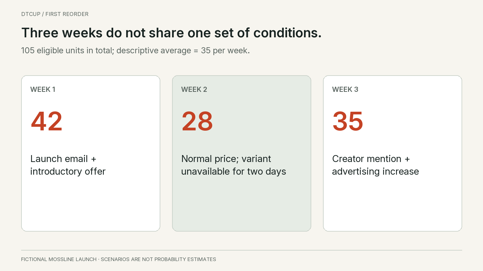
Mossline records 42 eligible order units in week one, 28 in week two and 35 in week three. Week one included a launch email and an introductory offer. Week two had normal pricing but a two-day period when a key variant could not be purchased. Week three included a creator mention and a modest advertising increase. The total is 105 units, but the three weekly numbers did not arise under identical conditions.
A simple average is 35 units per week. It is a useful descriptive starting point, not a stable demand estimate. The launch email may have concentrated existing interest into the first week. The unavailable variant may have suppressed some observed orders in the second. The creator mention may or may not produce a lasting effect. Extending 35 indefinitely assumes these influences combine into a repeatable future pattern.
Keep an event record beside the quantities. Note price, promotion, distribution, availability, traffic changes and known unusual orders. Do not write a elaborate explanation for every daily fluctuation. Record the events that could materially change the interpretation of the observed sales. The point is to avoid fitting a trend through operational changes while calling it organic demand growth.
Confirm the order definition before making adjustments. Exclude test transactions and duplicates under a documented rule. Keep refunds, cancellations and service replacements distinguishable. If you have not reconciled those quantities, start with the companion guide to building a usable demand history. A short series leaves little room for data errors; a few misclassified orders can materially change the apparent launch rate.
Do not convert the two unavailable days into a precise lost-sales estimate without supporting evidence. You can flag the week as constrained and explore a bounded adjustment, but the customers may have substituted another variant, returned later or abandoned the purchase. A simple daily-rate multiplication can be a scenario assumption. It should not be relabeled as observed demand.
Examine the order mix as well as the total. A large wholesale order, a group purchase or one unusually successful creator can dominate a small sample. That demand may be real and valuable, but it may not recur at the same pace. Keep it visible and decide whether the first-reorder baseline should treat it separately. Removing every spike is wrong; assuming every spike repeats is equally risky.
3. Choose several analogues and record why each might fail
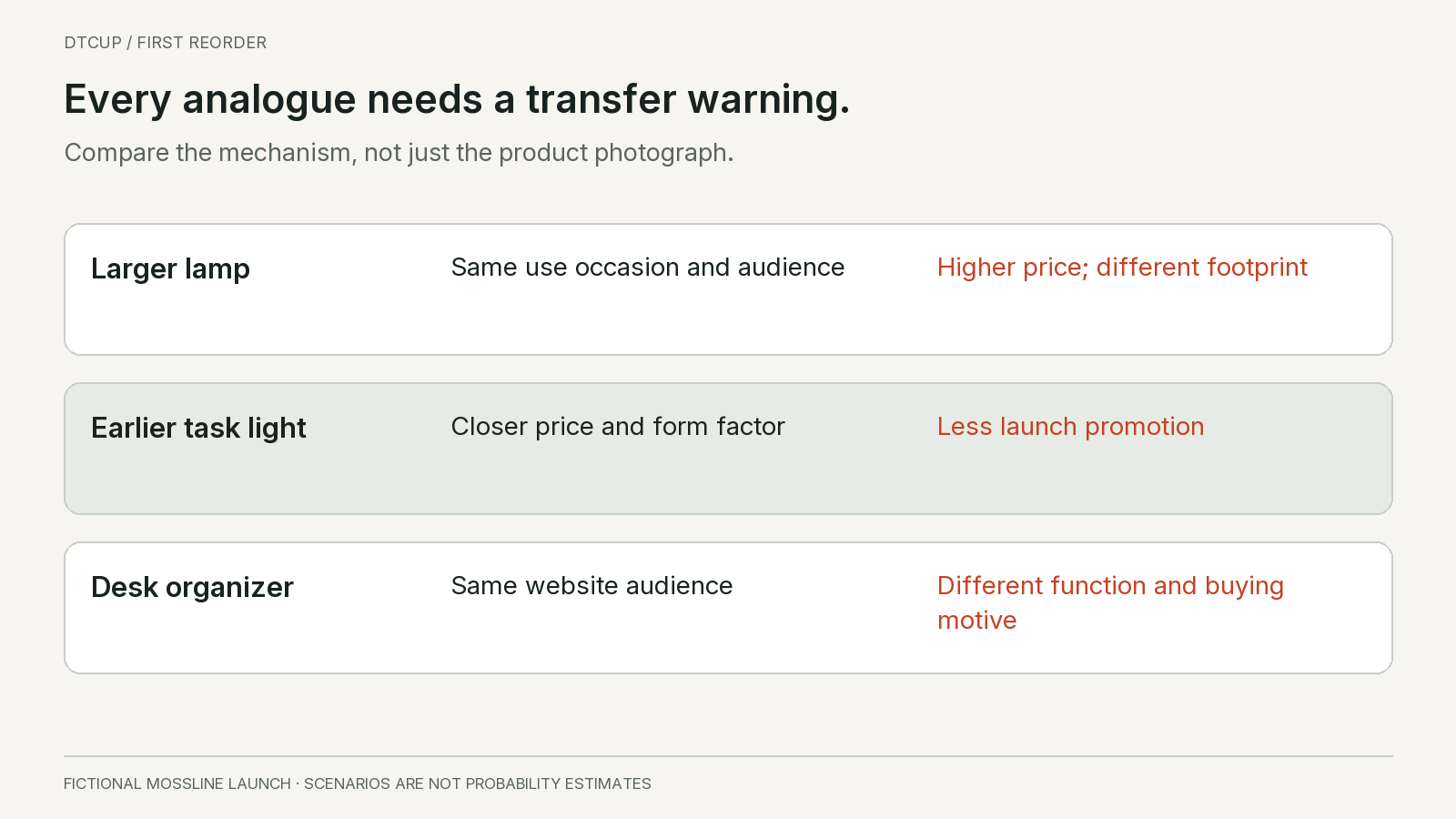
An analogue is a comparison used to inform judgment. It should not be a product selected because its growth story is attractive. For Mossline, the larger desk lamp shares the use occasion and brand audience, while a compact task light from an earlier launch shares the price range and form factor. A desk organizer shares the website audience but has a different function and purchase motivation. Each offers partial evidence.
Begin with similarities and differences before looking for a convenient average. Compare the launch channel, price, audience size, offer, availability, review base and marketing support. A previous product that launched to a large existing customer list may overstate the likely response for a product entering a new market. A product with a severe stockout may understate its own unconstrained demand.
The textbook discussion of forecasting by analogy recommends structured comparison across multiple analogies and attributes rather than relying on one convenient example. For a small brand, the practical version can be a short comparison sheet. Its value is making the reasoning reviewable, not creating a scientific-looking score from weak inputs.
Mossline chooses two primary analogues and one secondary reference. The larger lamp has useful repeat-purchase and consideration information but a higher price. The earlier task light has a closer price but received less launch promotion. The organizer helps estimate website audience exposure but is too different to determine conversion by itself. The team records these limitations beside any rates it borrows.
If you normalize by exposure, be precise about the denominator. Product-page sessions, qualified visits, email recipients and ad impressions are not interchangeable. A session can contain multiple page views, and the same person can visit repeatedly. A conversion rate from one channel mix may not transfer to another. Normalization can improve comparison only when the exposure definitions are sufficiently comparable.
Do not assign weights merely to make the final estimate land near a target. If the team gives the closer product more influence, explain which attributes justify that choice. Then test how the result changes under another reasonable weighting. A forecast that swings dramatically when a small judgment changes should be presented as fragile. Its apparent decimal precision does not make it robust.
Include failures and ordinary launches where relevant. Looking only at successful products creates an optimistic reference set. A product that underperformed because of a clearly different condition may deserve less weight, but it should not disappear simply because it is inconvenient. The goal is to understand a plausible range of outcomes, including the ways the new product could disappoint.
Finally, analogues should inform the first decision and then gradually give way to the product’s own evidence as that evidence becomes informative. There is no universal week when this handover must occur. It depends on volume, stability, changing exposure and the decision horizon. Keep the transition deliberate rather than treating the initial borrowed assumption as a permanent truth.
4. Build three explicit scenarios instead of one hidden compromise
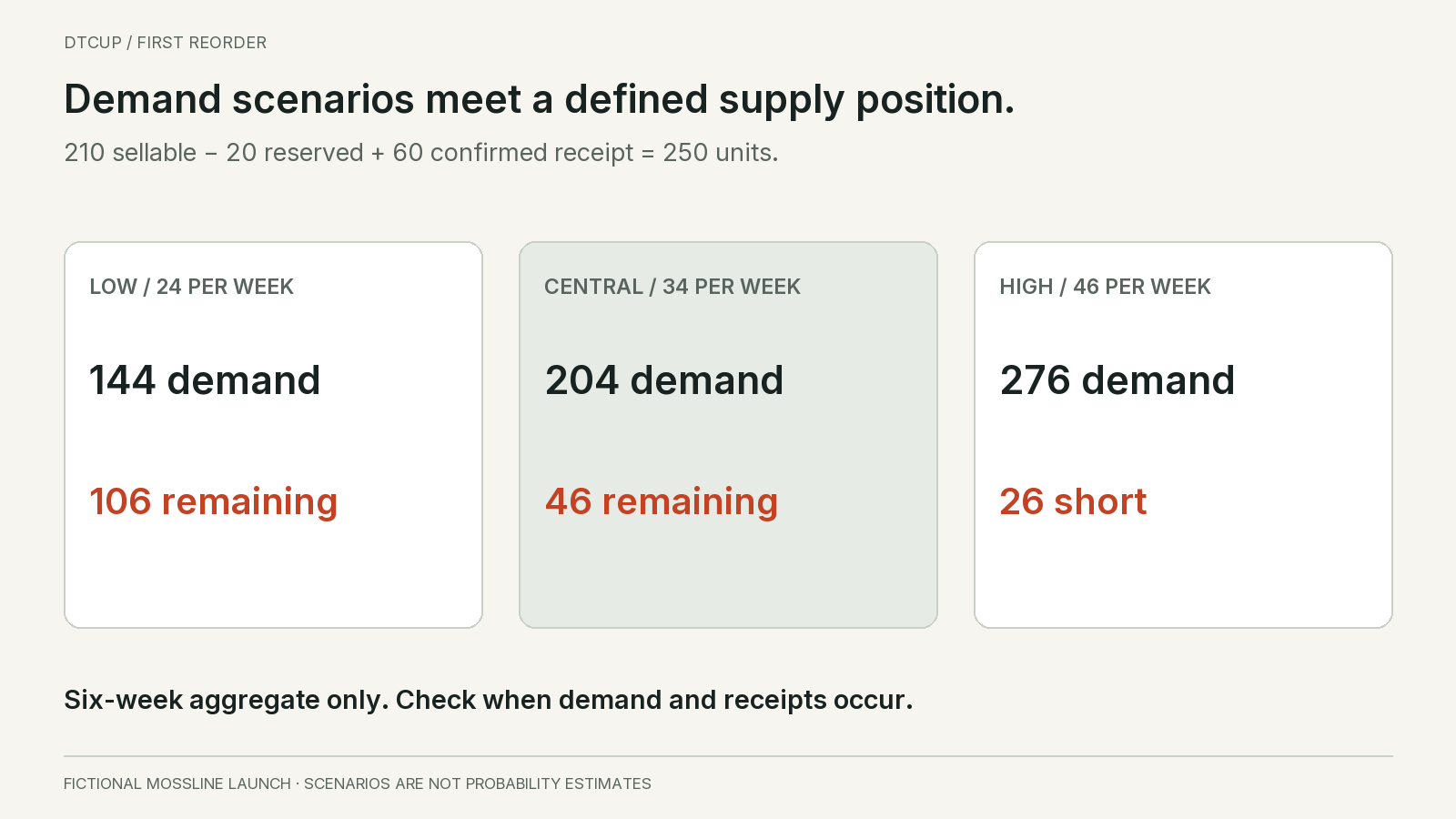
Mossline’s team selects illustrative weekly demand scenarios of 24, 34 and 46 units for the next six weeks. The low scenario assumes launch enthusiasm fades and ordinary demand settles below the observed average. The central scenario assumes the current audience and planned support sustain a rate near the early average. The high scenario assumes the creator activity and planned distribution broaden demand. These are judgmental scenarios, not statistically estimated percentiles.
Over six weeks, those rates imply 144, 204 and 276 units of new order demand. The arithmetic is straightforward; the important work is documenting the conditions behind each rate. A label such as “pessimistic” is less useful than “no further creator effect, normal price, planned email support only.” Conditions can be checked. A vague mood cannot.
Keep the scenarios internally coherent. If the high-demand case assumes a major advertising expansion, include the fact that this expansion must actually happen and be operationally feasible. If it assumes lower prices, the contribution per unit may change. If it assumes a new channel, onboarding timing and stock allocation matter. A high case should not combine every favorable outcome while ignoring the costs and constraints required to produce it.
Separate demand uncertainty from supply uncertainty. A six-week supplier lead time is not the same thing as a six-week demand scenario. If the receipt arrives two weeks late, the exposure period is longer. Explore that timing separately rather than burying it in a larger demand number. The team needs to know whether the risk comes from customer response or from the supply plan.
Do not attach probabilities unless there is a defensible basis for them. Writing 20%, 60% and 20% beside the scenarios can make a judgment exercise look calibrated when it is not. You may use explicit subjective probabilities in a decision process if the team understands and records their basis, but they should not be presented as model-derived confidence. For this example, we keep the cases unweighted and inspect the consequences of each.
A scenario range should be wide enough to include meaningful uncertainty but narrow enough to support action. If every imaginable outcome is included, the exercise becomes unhelpful. Use the analogues, observed conditions and planned activity to explain why these cases are decision-relevant. Then record which observations would cause the team to revise the range rather than treating it as fixed until the end of the season.
The central case is not automatically the purchase quantity. It is one demand assumption. Existing stock, open obligations, confirmed receipts, supplier minimums, cash and the cost of being wrong still stand between a demand scenario and an order. Keeping those layers separate is what makes the final commitment explainable.
5. Connect the scenarios to the actual supply position
At the review point, Mossline has 210 sellable lamp units physically available. Twenty are reserved for already accepted orders and should not be treated as free stock for future demand. There is a confirmed receipt of 60 units due in two weeks. For the simplified six-week calculation, the starting free position is 190 units and total supply available during the horizon is 250, assuming that receipt arrives on time and is sellable when received.
Against 144 units of new demand, the aggregate ending position is 106. Against 204, it is 46. Against 276, it is negative 26, indicating an aggregate shortage under those assumptions. These balances are not a service-level forecast. They summarize the six-week total and do not yet show whether a shortage occurs before the receipt arrives.
Check timing before interpreting the totals. With 190 units initially free and the largest weekly scenario at 46, the first two weeks require 92 units, so the example does not run out before the planned week-two receipt under a simple even-weekly timing assumption. A different daily pattern or delayed receipt could change that. The aggregate balance is a screening calculation; the time-phased view is what connects it to service risk.
Do not count reserved units twice. One valid approach starts with physical sellable stock and subtracts existing obligations plus future demand. Another starts with free stock after reservations and subtracts only future demand. Mixing the approaches can double-subtract the same orders or fail to reserve them at all. State which approach the worksheet uses and reconcile the opening quantity.
The inbound 60 also needs evidence. A purchase order date is not necessarily a delivery date. Production completion, transport, customs where relevant, receiving and inspection can all affect when units become sellable. Use the best verified expected date and a separate delay case. For a broader treatment of the supply timeline, see the existing guide to planning lead time through sellable stock.
If the new replenishment order placed today takes six weeks to arrive, it cannot solve a shortage that happens in week four unless another action changes the timeline. This seems obvious, but forecast sheets often add a proposed order to total supply without placing it on the calendar. A purchase quantity and an arrival date form one decision. Evaluating only the quantity can create a false sense of coverage.
6. Treat the first reorder as a commitment under uncertainty
The supplier offers a minimum order of 120 units in packs of 20, with an illustrative six-week lead time. Mossline cannot simply order the high case’s 26-unit shortage. A feasible order must respect the supplier terms and arrive when it can help. The buying decision therefore includes more than choosing the most likely demand number.
Consider the consequences of ordering 120 now. It creates additional future supply but also commits cash and storage capacity. If demand settles near the low case, that stock may cover a long period and reduce flexibility for other products. If demand remains high, 120 may be useful but still arrive too late to prevent a near-term shortage. The same order can be too much under one scenario and too late under another.
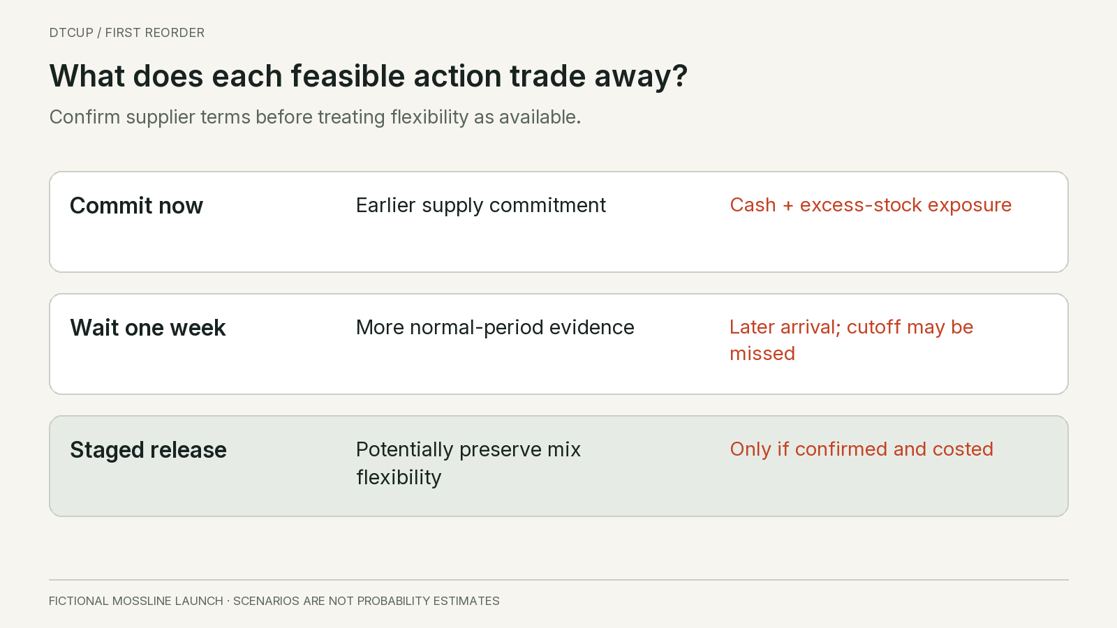
I would compare feasible actions rather than only quantities. Options might include the standard minimum order, a negotiated smaller release, a later commitment after another week of evidence, a split shipment, or an agreed capacity reservation. These are possibilities to discuss with a supplier, not terms every supplier will offer. Do not put an unconfirmed flexibility option into the plan as if it were guaranteed.
Each option has a cost of waiting and a cost of committing. Waiting can improve demand evidence but move the arrival date later. Ordering now can protect a future supply position but increase overstock exposure. A staged release can preserve flexibility if it is genuinely available, but may increase unit or freight cost. The decision should make those tradeoffs visible instead of hiding them in an arbitrary safety multiplier.
For a simple financial boundary, suppose each lamp ties up an illustrative $18 of landed inventory cost before selling expenses. A 120-unit order commits $2,160 under that limited cost definition. That number is not the full cost of the decision: payment timing, storage, financing, markdown risk and other costs may matter. It is a transparent starting point for discussing whether the business can afford the commitment if the low scenario persists.
Set the risk boundary with the responsible business owner. The planner should not assume the company wants zero stockouts at any inventory cost, or minimum inventory regardless of missed sales. A young brand with limited cash may rationally choose a different first order from an established brand with stable demand and flexible supply. The forecast informs that choice; it does not remove the need for judgment.
7. Decide whether another week of evidence is worth the delay
Waiting is valuable only if the information gained can change the decision enough to justify the later supply date. If the supplier’s minimum order remains 120 under every plausible scenario and the arrival date is already critical, another week may add little useful flexibility. If the next week includes a planned normal-price period without launch promotion, it may be unusually informative about the repeatable baseline.
Ask what observation would cause a different action. Mossline might decide that another week near the low case, under full availability and normal exposure, would support delaying the standard reorder. A week near the high case with broad order distribution across days and sources might support committing sooner. A single large one-off order would be treated separately. These are illustrative review rules, not universal numerical thresholds.
The observation must be interpretable. A low week during a payment outage is not strong evidence that demand faded. A high week after a deep discount is not direct evidence of normal-price demand. Record whether the expected learning conditions actually occurred. Otherwise the team may wait for information, receive a confounded result, and still act as if uncertainty has been resolved.
There is a practical distinction between postponing a decision and preserving an option. Asking the supplier whether capacity can be reserved without a full release, whether materials are shared with another product, or whether a smaller first delivery is possible can change the tradeoff. These options have value only when confirmed and costed. A casual “we can probably arrange it” should not support a service commitment to customers.
Use a decision deadline. If production slots close on Friday, the review must happen before Friday with the evidence available then. A forecast process that continually asks for one more week can miss the only feasible replenishment window. The purpose of uncertainty analysis is to make a timely, explainable choice, not to postpone responsibility until uncertainty disappears.
I would summarize the information question in the reorder brief: what we expect to learn, which action it could change, the last date that action remains available, and the cost if we wait. That forces the team to connect analysis to the supplier calendar. It also prevents a busy dashboard from becoming a substitute for a decision.
8. Use early indicators as context, not as converted orders
A new product can generate waitlist signups, product-page visits, saves, customer questions and positive survey responses before it produces stable order history. These signals can be useful, but they represent different levels of commitment. Ten people saying they like the lamp are not ten future purchases. A waitlist built with a strong incentive may behave differently from one built through ordinary product interest.
Connect each signal to a specific uncertainty. Repeated questions about dimensions may indicate that the product page does not make size clear. Strong add-to-cart activity followed by weak checkout completion may suggest a purchasing friction or an offer mismatch. Neither observation should be converted into missing unit demand without a defined method and evidence. Use the signal to investigate, not to inflate the forecast automatically.
Preorders are stronger commitments than casual interest when they are genuine accepted orders under the business’s rules, but they still need cancellation and fulfillment context. A preorder backlog can represent demand accumulated over a long announcement period. Treating that backlog as a recurring weekly run rate can greatly overstate the steady state. Separate the accumulated commitment from the ongoing arrival of new orders.
Customer feedback can improve the scenario assumptions. If buyers consistently choose the compact lamp for small desks rather than as a cheaper replacement for the large lamp, that changes the substitution hypothesis. If many buyers mention a temporary creator recommendation, the team should consider whether the exposure will repeat. Feedback explains mechanisms; it does not automatically provide a representative conversion rate.
Keep the denominators visible when using rates. A conversion rate based on 40 highly engaged launch-email visitors may not transfer to thousands of cold advertising visitors. A small numerator also produces substantial uncertainty. Avoid treating a percentage displayed to two decimals as more reliable than the underlying counts. Report the counts and the acquisition context beside the rate.
There is a useful hierarchy of questions: what did people actually order, under what conditions, what prevented additional orders, and what evidence suggests future conditions will differ? Early indicators belong mainly in the last two questions. They enrich the planning judgment without being silently added to the observed-order history.
9. Forecast the product family before pretending every variant is stable
A launch with several colors or sizes can fragment a small amount of evidence into even smaller series. If Mossline sells 105 units across four finishes, one finish may have only a handful of orders. Fitting a separate complex model to each variant creates an illusion of specificity. The purchasing decision may be better served by a family-level scenario and an explicit, revisable mix assumption.
Check availability before interpreting the mix. If the sand finish was unavailable for two days, its observed share may be suppressed. Customers may have switched to another finish, waited, or left. The resulting shares are not a clean preference survey. Preserve the availability condition and avoid locking the initial mix into a large purchase without acknowledging that limitation.
Use comparable-product mix cautiously. A finish popular on a large lamp may not have the same appeal on a compact model. The product photography, intended room and price can change preferences. An analogue can provide a starting allocation, but it should be treated as an assumption and reviewed against the new product’s own unconstrained orders where possible.
For illustration, a 120-unit supplier minimum with 20-unit pack increments might allow 40 units of one finish, 40 of another and 20 each of two others. That is a feasible mix, not an optimal one established by three weeks of data. If the supplier requires a minimum per finish, the total commitment may become much larger. The planning brief should use the actual feasible combinations rather than rounding each independent variant forecast upward without inspecting the combined excess.
Review the category total as well. If compact-lamp sales rise while the larger lamp declines, the net category change may be smaller than the new SKU’s sales suggest. That could be healthy customer choice rather than a problem. But replenishing both products as if each retained its old independent demand can create surplus. Track the substitution hypothesis explicitly and look for evidence over a suitable period.
Shared components can offer another form of flexibility if the supply process permits it. A common base or packaging component may be stocked before the final finish mix is committed. Do not assume this is possible; confirm production constraints and costs. When it is feasible, postponing variant commitment can reduce the risk created by an uncertain early mix more effectively than trying to estimate each variant with false precision.
10. Update the forecast without chasing every daily movement
Short history deserves frequent attention, but frequent attention is not the same as rewriting the forecast after every order. Choose a review cadence that matches the decision and supply process. Daily checks may be appropriate for stock availability and obvious data problems. A weekly planning review may be more useful for revising scenarios and commitments, unless a material event requires earlier action.
At each review, compare the new observation with the scenario conditions, not just the central number. If week four records 31 units under normal price and full availability, it provides different information from 31 units during a two-day outage. If the creator campaign did not happen, the high-case condition was absent. The team should update the assumption that changed rather than treating every miss as evidence that the whole method failed.
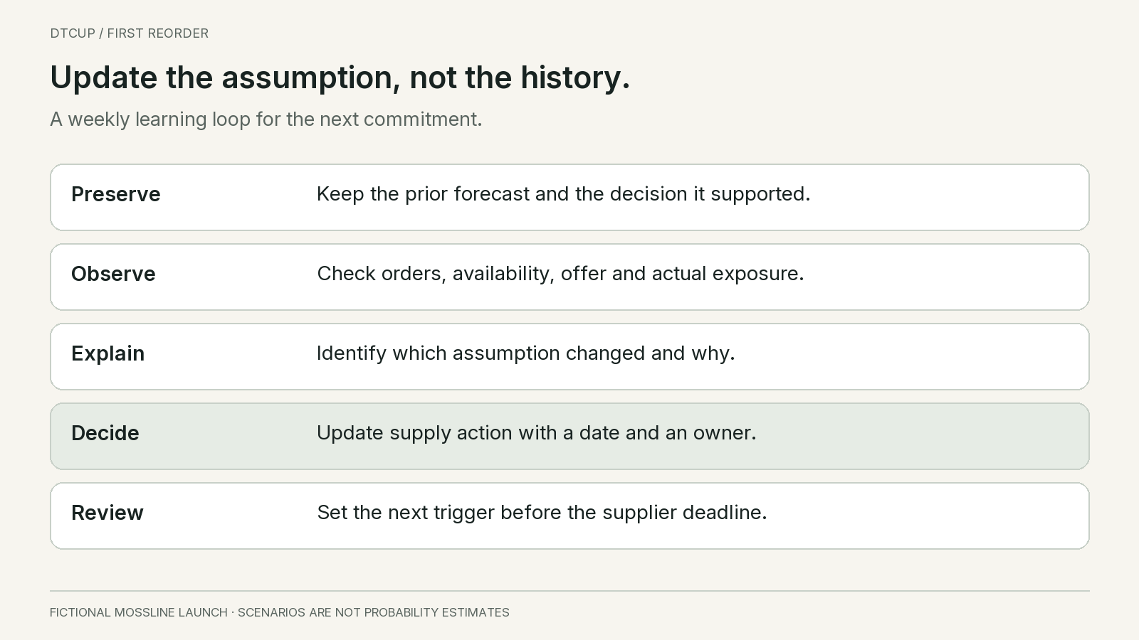
Keep the previous forecast version. Record its date, horizon, scenarios, known stock position, expected receipts and chosen action. Then add the new version rather than overwriting the old one. This allows the team to distinguish a poor assumption from a later change in circumstances. It also makes it possible to learn whether recurring optimism, pessimism or late supply updates are driving avoidable errors.
Use a reason code in plain language for each material adjustment. Examples include normal-price demand below expectation, new channel launch confirmed, source coverage corrected, supplier delay, or variant availability restored. A forecast changed “because sales changed” is not a sufficient explanation. The relevant question is why the new evidence changes the expectation for the remaining decision horizon.
Do not demand accuracy from a scenario that did not describe the realized conditions. If the high scenario assumed a campaign that never ran, comparing actual orders with that scenario as if it were an unconditional prediction is misleading. You can still review whether the campaign assumption was reasonable, but that is a planning-assumption review rather than a pure model-error calculation.
As evidence accumulates, compare simple baselines. A recent average, a normal-period average and a carefully chosen analogue may be enough to create useful benchmarks. More advanced methods should earn their place by improving relevant decisions under an honest evaluation, not by producing a more impressive chart. With very short history, the available evidence may be insufficient to distinguish methods reliably.
Seasonality requires particular restraint. Three weeks cannot establish a recurring annual pattern for the new product. You may use category or analogue evidence to construct a seasonal hypothesis, but label it as borrowed information and examine whether the mechanism transfers. A launch in November does not prove the product always peaks in November. The launch timing and the seasonal pattern are entangled in the observation.
11. Write a first-reorder brief another person can challenge
Before signing the brief, check whether the planned offer is the same offer the observations describe. Suppose Mossline intends to raise the price after launch and remove free delivery. The early unit rate was measured under different customer economics. The team should not carry the rate forward unchanged while simultaneously improving the assumed margin. That would combine the demand response of one offer with the profitability of another without evidence that customers will behave the same way.
A practical response is to make the offer change explicit in the scenarios and use the next normal-price period to learn. Record the dates, exposure and availability conditions so the comparison remains interpretable. If several things change together, acknowledge that the observed difference cannot be assigned neatly to price alone. This does not prevent a decision; it prevents the team from claiming a precise price response that the launch data cannot support. The resulting reorder can still be bounded by cash, supplier flexibility and a scheduled review.
The brief can be short even when the analysis behind it is careful. Begin with the exact decision and deadline: whether to place a feasible replenishment order for the compact lamp before the supplier’s production cutoff. State the latest verified free stock, existing obligations, confirmed receipts and expected sellable dates. Identify any source limitations that could change those quantities.
Then summarize the observed launch history and its conditions. For Mossline, that means 42, 28 and 35 eligible units across three differently supported weeks. State that the 35-unit average is descriptive and that the constrained week has not been converted into a precise lost-demand estimate. List the analogues used and the main reason each may fail to transfer.
Present the low, central and high cases with their conditions and consequences. In our example, six-week demand is 144, 204 or 276 against an aggregate available position of 250 under the stated timing assumptions. The brief should show the shortage or residual inventory consequence, then connect it to feasible supplier actions. Do not let a negative aggregate balance imply that an order arriving at the end of the horizon can repair an earlier shortage.
Record the selected action and the reason it is acceptable under uncertainty. The action might be a standard commitment, a confirmed staged release or a deliberate wait with a deadline. There is no single correct choice established by the fictional numbers alone. The decision depends on costs, service priorities, cash, flexibility and the owner’s risk boundary. The article provides the reasoning structure, not a purchase instruction for a real business.
Include the evidence that would trigger a review before the next scheduled meeting. A supplier delay, a sustained rate outside the scenario range under comparable conditions, a major product defect, a channel launch or a corrected inventory count could all matter. Use triggers tied to consequences rather than reacting to every normal fluctuation.
Finally, assign ownership. Someone verifies source quantities, someone confirms supply dates, someone owns the demand assumptions, and someone authorizes the financial commitment. In a small company, one person may hold several roles. Naming the responsibilities still helps prevent a forecast number from being treated as approval to place an order.
12. Judge the first cycle by what the business learned and protected
The first replenishment cycle will rarely reveal a perfectly stable demand rate. It can still produce a good decision. The business may avoid an unaffordable commitment, preserve a useful supply option, discover a variant preference, or identify that launch demand was concentrated in an existing audience. These are valuable outcomes even when the central forecast misses the final total.
Review the decision using the information available at the time. Did the team define the unit correctly, identify the launch conditions, consider plausible downside, verify supplier constraints and set a timely review? Did new evidence arrive that reasonably changed the plan? A lucky outcome from an unsupported assumption should not be celebrated as a repeatable method, and an unlucky outcome under a well-reasoned risk choice should not automatically invalidate the process.
Separate demand error, supply error and execution error. Demand may differ from the scenario. A shipment may arrive late. The team may fail to place an approved order before the cutoff. Those are different problems with different owners. A single “forecast accuracy” percentage can conceal the operational issue that actually caused the shortage or excess stock.
My advice is to make the first forecast modest in its claims and strong in its decision logic. Use the early history honestly, borrow from analogues with visible limitations, keep scenarios separate from probabilities, and connect every purchase quantity to a date and a risk boundary. The aim is not to know the product’s future after three weeks. It is to make the next commitment in a way the business can understand, afford and improve.
Sources
Still have a question?Ask the DTCUP Community ↗