
MOQ and Pack Sizes: When a Cheaper Unit Creates Expensive Inventory
Compare feasible purchase quantities with the cash and stock they commit. A worked example shows when a volume discount loses, when it wins and which revised offer changes the tradeoff.

7 years of experience building and operating brand websites, specializing in website development, paid advertising and SEO. Built a brand website from launch to US$10 million in annual sales.
The Short Answer
First calculate feasible quantities from the actual minimum and pack rule. Compare complete purchase cash, dated affordability, demand served and the treatment of leftover units. A discount is worthwhile only within a feasible option whose additional stock and uncertainty the business can justify.
Key takeaways
- Keep the original requirement separate from pack rounding.
- A lower unit cost can require substantially more initial cash.
- Leftover recovery and its timing must be explicit.
- A larger order can win when it serves otherwise lost demand.
- Expected return cannot pay an earlier invoice.
- A revised supplier offer must be evaluated across the same scenarios.

The cheapest unit can belong to the most expensive purchase decision. A supplier reduces the price if you buy more, the spreadsheet shows a better margin, and the extra cartons seem harmless until they occupy cash that another product needs. The mistake is usually not arithmetic. It is calculating the saving on units you expect to sell while avoiding a decision about the units you must also buy.
I would evaluate a minimum order as a complete, feasible commitment. First establish the quantities the supplier will actually accept. Then compare cash timing, service consequences and the likely use of leftover stock. A lower price matters, but it belongs inside that comparison. It should not be the conclusion before the quantity and selling horizon are understood.
This article builds a worked purchasing model for fictional Juniper Case, a brand buying a seasonal accessory. Every quote, demand scenario, recovery value and cost is an invented teaching assumption. The example is not a supplier offer, accounting policy or benchmark. Its purpose is to show which calculations change the decision and how to expose the assumptions that deserve investigation.
Turn a requirement into feasible quantities
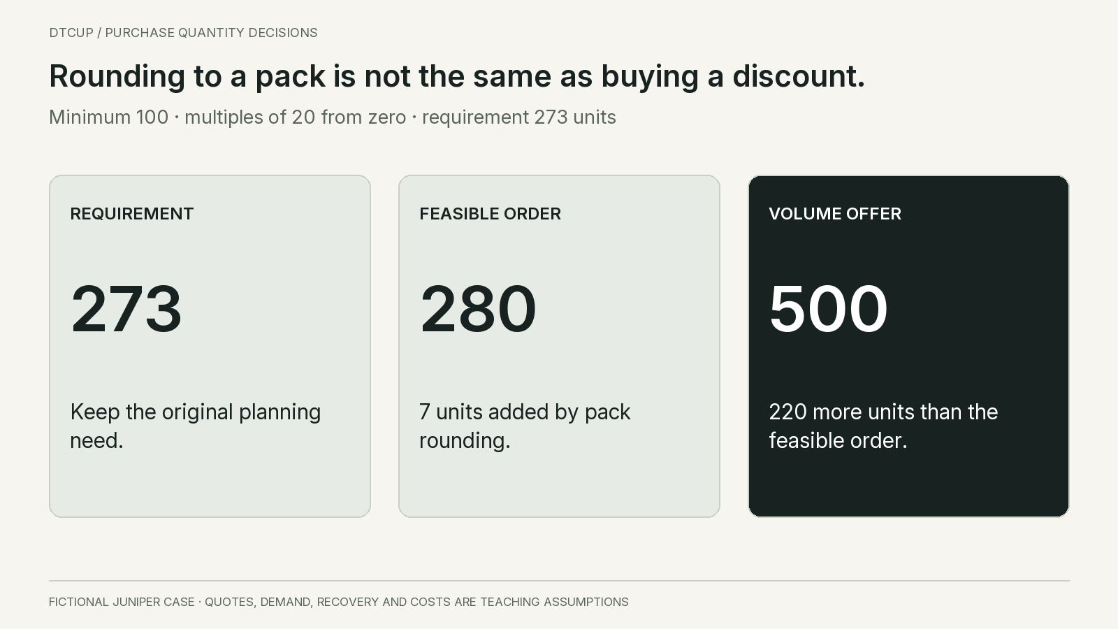
A replenishment calculation might suggest buying two hundred seventy-three units. That does not mean the supplier will accept an order for that quantity. A minimum order and a pack multiple create a set of feasible choices. If the minimum is one hundred units and purchases must be multiples of twenty, the smallest feasible quantity at or above the requirement is two hundred eighty.
State the convention before writing a formula. In this example, the ordered quantity must be at least the minimum and must be a multiple of the pack size measured from zero. Divide the larger of requirement and minimum by the pack size, round upward to an integer, and multiply by the pack size. If the supplier instead allows increments above a special first quantity, the formula changes. Confirm the rule rather than assuming every minimum behaves identically.
For a requirement of ninety-three units, a minimum of one hundred and a pack size of twenty, the feasible starting point is one hundred. For a requirement of one hundred three, the starting point is one hundred twenty. If the minimum were one hundred ten while multiples of twenty still applied from zero, the first feasible quantity would also be one hundred twenty. These small examples expose ambiguities that a polished purchasing dashboard can conceal.
Now separate quantity feasibility from decision quality. Rounding two hundred seventy-three to two hundred eighty adds seven units. Raising the purchase to five hundred to reach a discount adds two hundred twenty units beyond the rounded requirement. Those are different choices. The first satisfies the supplier’s packaging rule; the second accepts a larger commercial exposure in exchange for a different price.
Check whether constraints apply per variant, across a family or to an entire order. A combined minimum does not imply that the supplier accepts any mix. Four colors with a separate minimum of one hundred each create a different commitment from a four-hundred-unit total that can be allocated freely. Write quantities at the level where the constraint actually applies so that a strong seller cannot hide an unwanted color inside the total.
Finally, preserve the unrounded requirement. It helps the team see how much stock comes from expected use and how much comes from a supplier constraint or an intentional buffer. Calling the entire order “forecast demand” erases the reason for the excess. That makes the next forecast look wrong when the original purchasing decision deliberately exceeded it.
Compare quotes on one cost boundary
Juniper Case has no starting stock in this simplified decision. It is comparing one initial purchase for a twelve-week selling period. Both suppliers meet the same approved product specification, and all units are assumed to be usable before selling begins. There is no replenishment within the period. These assumptions deliberately remove quality and lead-time differences so the quantity tradeoff is visible; a real comparison must put those differences back.
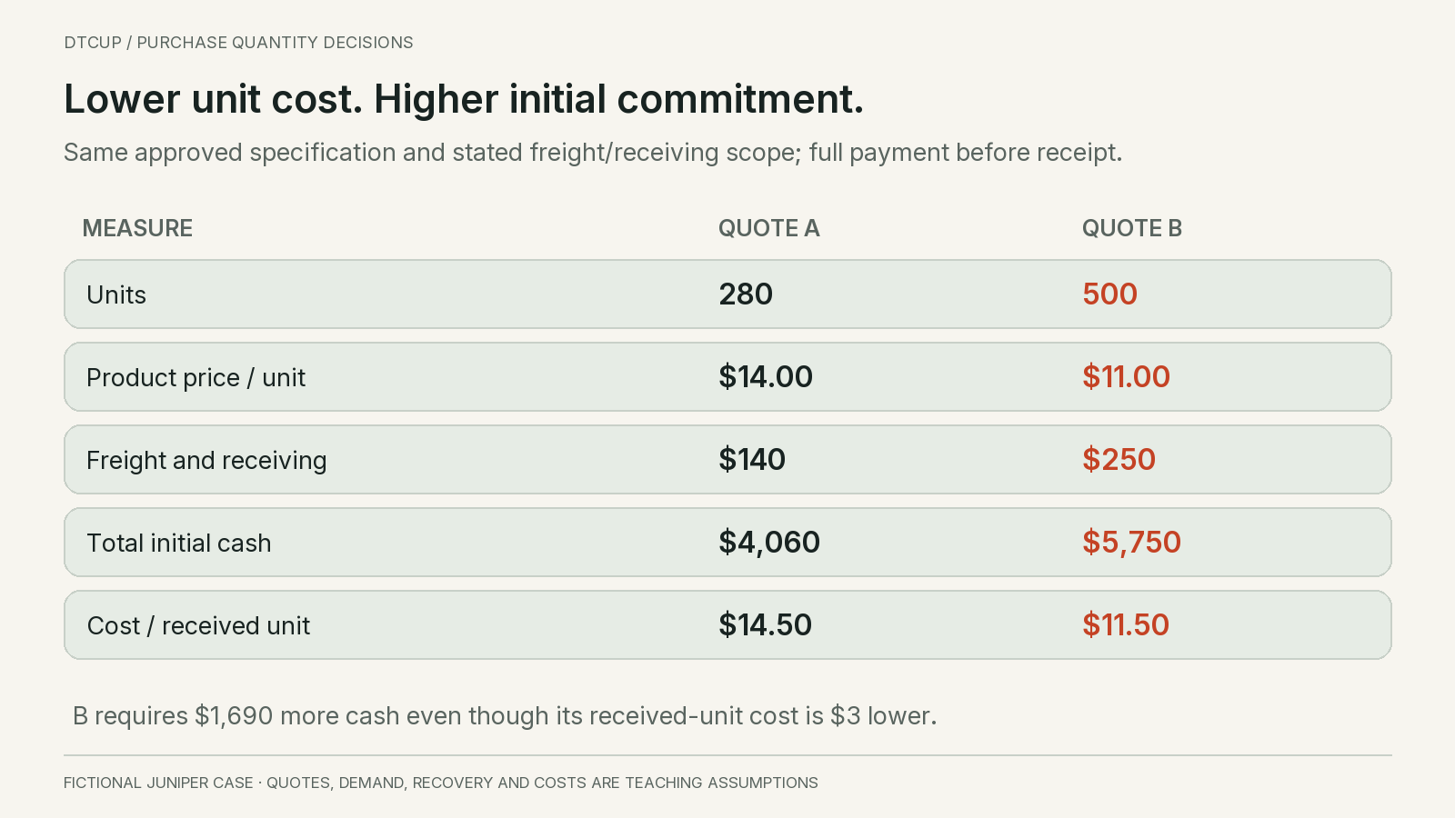
Quote A allows the two-hundred-eighty-unit order. Its product price is fourteen dollars per unit, with one hundred forty dollars for the agreed freight and receiving scope. The total initial cash requirement is four thousand sixty dollars: two hundred eighty times fourteen, plus one hundred forty. The cost per received unit for this stated scope is fourteen dollars and fifty cents.
Quote B requires five hundred units at eleven dollars each, plus two hundred fifty dollars for the same freight and receiving boundary. Its total initial cash requirement is five thousand seven hundred fifty dollars, or eleven dollars and fifty cents per received unit. The unit figure is three dollars lower than A, but the initial payment is one thousand six hundred ninety dollars higher.
Do not call either number a complete landed cost unless the relevant costs have actually been included. The International Trade Administration’s landed-cost explanation includes product cost, freight, insurance, tariffs, taxes and other applicable fees. For a real shipment, confirm responsibilities and current estimates with the appropriate specialists. Our fictional comparison uses only its explicitly stated purchasing scope and assumes any other relevant differences have been resolved before approval.
Payment timing is another column, not a footnote. For the first comparison, assume the full quoted amount is paid before stock becomes usable. A deposit credited against the balance is part of that total, not an additional cost. A later payment term can change the lowest cash point without changing the product amount. Record both the total obligation and the dates on which cash leaves.
Also clarify whether a discount applies to every unit or only to units above a threshold. Five hundred units at an all-units price of eleven dollars cost five thousand five hundred before other charges. A marginal discount on only the units above a threshold produces a different total. Do not apply the lower price to the whole order unless the written offer supports that interpretation.
Account for the extra units before celebrating the saving
At the base selling assumption of two hundred eighty units, both quotes can serve the same customer demand. A buys exactly that quantity. B leaves two hundred twenty units after those sales. To compare the options, the team needs a stated treatment of that remaining stock. Leaving it out implicitly assumes it has no consequence; valuing it at full retail implicitly assumes a future sale that has not been established.
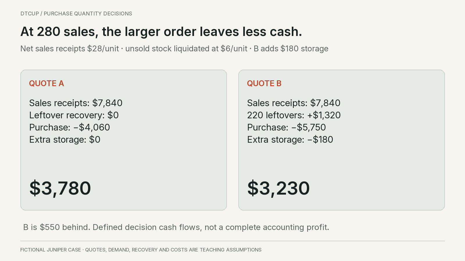
For this example, each unit sold during the period produces twenty-eight dollars of net receipts after the selling costs included in that measure, but before the purchasing costs shown above. Assume unsold units are liquidated at period end for six dollars each net of the costs of that liquidation. Quote B also requires a fixed one-hundred-eighty-dollar reservation for extra storage capacity during the period. Common operating costs are excluded from both options.
The storage charge is a specific incremental fee in the example, not a universal holding-cost percentage. It applies to B under each scenario because the extra capacity is reserved when the purchase is made. If your warehouse charges by actual daily volume, model that schedule instead. Defining the fee this way prevents the arithmetic from quietly changing when the demand scenario changes.
Under A, two hundred eighty sales generate seven thousand eight hundred forty dollars. Subtract the four-thousand-sixty-dollar purchase and the decision-scope net cash surplus is three thousand seven hundred eighty dollars. Under B, the same sales generate seven thousand eight hundred forty, the two hundred twenty leftovers recover one thousand three hundred twenty, and purchase plus extra storage costs five thousand nine hundred thirty. The resulting surplus is three thousand two hundred thirty dollars.
B is therefore five hundred fifty dollars worse under these assumptions, despite its lower unit cost. This is a comparison of defined cash flows through an assumed liquidation, not an accounting profit statement. It does not include common overhead, income taxes or unlisted costs. The commercial lesson does not require calling the number profit: the cheaper unit leaves less cash from the stated decision in this base case.
There is another way to check the result. B saves three dollars on each of the two hundred eighty units that A would have bought, a saving of eight hundred forty. Its extra two hundred twenty units cost two thousand five hundred thirty at the allocated eleven-dollar-fifty cost. Subtract the eight-hundred-forty saving and the extra initial payment is one thousand six hundred ninety. Recover one thousand three hundred twenty from leftovers, subtract the one-hundred-eighty storage fee, and B remains five hundred fifty behind.
The second calculation is a useful reconciliation, not an independent benefit to add again. Counting the eight-hundred-forty saving on top of the first cash comparison would double-count it. Keep one primary model and use alternative calculations to verify the same result. A purchasing presentation should make the tradeoff easier to inspect, not multiply favorable numbers describing the same saving.
Change demand and see what reverses the decision
A larger order is not automatically wrong. It can protect sales that the smaller order cannot serve. The comparison should show that benefit rather than describing every unsold unit as a mistake. Juniper Case considers three hypothetical demand levels during the same twelve weeks: one hundred eighty, two hundred eighty and four hundred units. These are scenarios, not probabilities estimated from customer data.
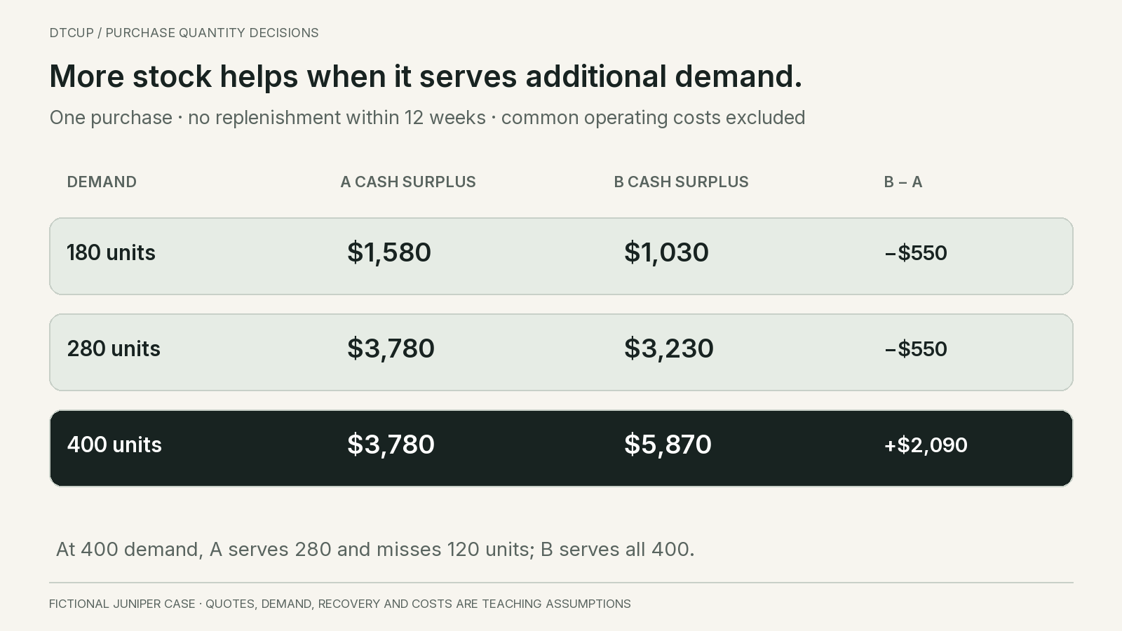
At one hundred eighty units of demand, A sells one hundred eighty and liquidates one hundred. Its net receipts are five thousand forty from sales plus six hundred from liquidation, less four thousand sixty for the purchase. The result is one thousand five hundred eighty. B sells the same one hundred eighty, liquidates three hundred twenty for one thousand nine hundred twenty and subtracts its purchase and storage costs. Its result is one thousand thirty, again five hundred fifty lower.
At four hundred units of demand, the difference changes. A can sell only two hundred eighty because the example allows no replenishment inside the period. Its cash result stays at three thousand seven hundred eighty, while one hundred twenty units of demand go unserved. B sells four hundred for eleven thousand two hundred, liquidates one hundred for six hundred and subtracts five thousand nine hundred thirty. Its result is five thousand eight hundred seventy.
In the high-demand scenario, B is two thousand ninety ahead and serves one hundred twenty more units. That improvement is not merely a lower purchasing cost. It includes additional fulfilled demand. If those extra sales require extra advertising, labor or delivery expense beyond the twenty-eight-dollar receipt definition, the model must include those differences. Otherwise the larger order receives credit for revenue while avoiding the costs needed to obtain it.
The unserved units in this example are lost sales within the period, not a backlog that later receives stock. Changing that assumption changes both cash timing and customer consequences. Record whether customers wait, substitute or leave before applying this comparison to your own purchase.
The scenario table gives the buyer a sharper research question: how plausible is demand above the smaller order’s capacity within the period? It also reveals an alternative question: can the business arrange a timely second order instead of committing to five hundred now? That alternative is outside the initial one-purchase model and should be evaluated explicitly, not smuggled in as an optimistic assumption for A.
If the team wants an expected-value calculation, it needs defensible scenario weights or a clearly labeled sensitivity exercise. For illustration only, weights of twenty percent low demand, sixty percent base and twenty percent high produce a weighted surplus of three thousand three hundred forty for A and three thousand three hundred eighteen for B. The twenty-two-dollar difference is tiny relative to uncertain recovery values and operating assumptions. It is not evidence of a precise forecast.
Because B is five hundred fifty behind in the two lower scenarios and two thousand ninety ahead in the high one, its weighted advantage changes sign when the assumed high-scenario weight exceeds about twenty-point-eight percent, holding this simplified two-outcome difference structure fixed. That threshold is a sensitivity result, not a measured probability. It tells the team which belief is driving the choice and how little confidence a close expected-value ranking deserves.
Test cash feasibility before ranking expected returns
Suppose Juniper Case has a verified five-thousand-dollar limit available for this purchase after protecting its other operating commitments. With full payment required before receipt, A fits the limit and B does not. B’s possible later sales or liquidation proceeds cannot pay an earlier invoice. The business either needs a genuinely different payment arrangement or must exclude B from the currently feasible set.
This is why I would not present a financially infeasible option as the recommended purchase and leave “finance to confirm” at the bottom. The constraint belongs in the decision model. If a financing proposal becomes available, include its actual cost, conditions and timing, and assess it with the responsible finance owner. Do not assume that short-term funding is free or available merely because a spreadsheet needs the order to work.
Draw a dated cash timeline. Start with the approved opening balance, subtract deposits and balances when due, include freight and other payments at their actual milestones, and add customer receipts according to realistic settlement timing. The lowest balance matters. A positive end-of-period result can coexist with an earlier inability to pay a necessary bill.
Keep the purchase allocation distinct from total cash in the bank. Payroll, taxes, refunds, other purchase orders and basic operations may already claim part of that balance. This article does not prescribe a universal reserve. It asks the operator to use the business’s approved constraints instead of treating all visible cash as available for a volume discount.
Also inspect concentration. A feasible order can consume nearly all flexible purchasing capacity in one uncertain item. The opportunity cost is not automatically the revenue of another product; it is the best credible use of the constrained resource that the larger order displaces. Identify that alternative concretely. “We might need the cash” is vague, while “this prevents the already-approved replenishment of the core size next week” is a decision-relevant consequence.
Finally, distinguish an attractive commercial case from permission to execute. The buyer can prepare the analysis, but the order should follow the business’s approval process. Record whether the option is proposed, approved, ordered, paid, received or released for sale. Those states prevent a supplier discussion or a favorable calculation from being mistaken for a completed commitment.
Make leftover value a defensible assumption
The six-dollar recovery value carries much of the base-case result. It should therefore be visible, dated and challenged. A liquidation estimate is not the normal retail price, the supplier’s original invoice value or the amount the team hopes to recover. It is an estimate of cash obtainable through a specified route after the costs required to use that route.
For Juniper Case, the hypothetical route might be a clearance buyer purchasing the remaining accessory at period end. The estimate should specify which condition, packaging, quantity and timing it assumes. If the buyer accepts only unopened cartons, a partly sold assortment may qualify differently. If the quote is nonbinding, the uncertainty remains. Do not make the value look guaranteed by entering it with two decimal places.
Test a lower recovery without changing anything else. At zero recovery, A’s base-case result stays three thousand seven hundred eighty because it has no leftovers at two hundred eighty sales. B’s result becomes one thousand nine hundred ten: seven thousand eight hundred forty less five thousand seven hundred fifty and one hundred eighty. The disadvantage grows to one thousand eight hundred seventy. That is the amount the team is exposed to if the assumed recovery route fails under this base scenario.
The break-even recovery value for B in the base case is eight dollars and fifty cents per leftover unit. B needs to recover its extra initial payment of one thousand six hundred ninety plus the one-hundred-eighty storage fee across two hundred twenty remaining units. Dividing one thousand eight hundred seventy by two hundred twenty gives eight dollars and fifty cents. Compare that requirement with evidence of achievable net recovery, not with the normal selling price.
Alternatively, the business may intend to retain the leftovers and sell them later. That requires a longer horizon with future demand, future selling costs, additional carrying costs and possible product changes. It is a different model. Do not combine a short selling period with an assumed full-value ending asset and describe the result as cash returned to the business.
Accounting treatment should also remain separate from management assumptions. Inventory valuation, write-downs and recognized profit follow the business’s applicable accounting rules and responsible professional review. This operational model estimates specified cash consequences. Calling a speculative future recovery “inventory value” does not establish an accounting amount, and an accounting carrying amount does not guarantee that cash can be recovered on the planned date.
Avoid double-counting the cost of holding stock
Holding cost is useful only when the team can explain what it includes. A broad annual percentage may combine capital, storage, insurance, damage and obsolescence assumptions. If the model then separately subtracts a storage fee and a liquidation loss, it may charge the same consequence twice. Conversely, using only warehouse rent can omit the cost of financing or handling excess stock.
For the worked example, the extra one-hundred-eighty-dollar fee is the only incremental storage charge included. The lower terminal recovery already captures a specific reduction in the cash recovered from unsold units relative to their purchase cost. We have not added a separate obsolescence percentage or financing charge. That makes the scope narrow but inspectable. A real model can be broader, provided each added component represents a distinct cost.
If storage is charged by unit-days, use the projected daily stock path. Five hundred units arriving together and declining through the season create a different usage pattern from staged receipts. Average starting and ending stock can be a reasonable approximation under a stated smooth-depletion assumption, but promotions, partial deliveries and stock transfers can make that shortcut poor. The relevant detail is the cost driver, not the most elaborate formula available.
If the cash cost depends on actual borrowing, apply the verified rate and dates to the relevant balance. If the business uses an internal opportunity-cost assumption, label it as a decision assumption rather than an invoice. These two approaches can support different questions. Combining both without explaining their relationship risks counting capital cost twice.
Also distinguish fixed and avoidable costs. An existing warehouse lease may not change when the order increases, while an extra pallet reservation or temporary overflow charge does. For the choice between two orders, identify the costs that differ. For a broader business profitability review, include the full relevant cost structure. A decision comparison and a complete operating statement need not use the same boundary.
Keep a cost dictionary beside the model. For each amount, write its unit, timing, source, whether it changes between options and whether another line already captures it. This is often more valuable than adding another decimal place to a carrying-rate assumption. It allows someone who did not build the spreadsheet to reproduce the result and challenge the inputs that matter.
Price flexibility as a real alternative
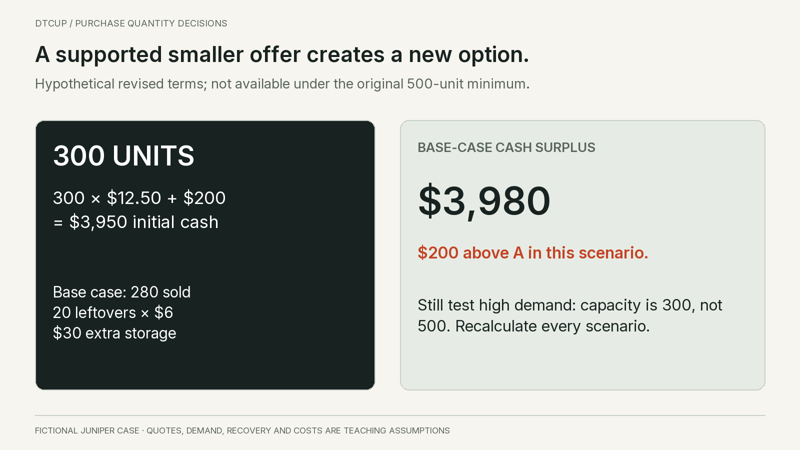
The first two quotes are not necessarily the only possible choices. After reviewing the base-case exposure, Juniper Case asks for a supported three-hundred-unit arrangement. Assume the supplier provides a new written offer at twelve dollars and fifty cents per unit plus two hundred dollars for the same freight and receiving scope. The total is three thousand nine hundred fifty. This is a hypothetical new offer, not a quantity available under B’s original five-hundred-unit minimum.
At two hundred eighty sales, the revised option leaves twenty units. At the same six-dollar net recovery, those return one hundred twenty dollars. Suppose the smaller additional storage requirement costs thirty dollars. The decision-scope surplus is seven thousand eight hundred forty plus one hundred twenty, less three thousand nine hundred fifty and thirty: three thousand nine hundred eighty dollars. That is two hundred higher than A in the stated base case.
The revised offer also fits the five-thousand-dollar initial purchase limit. However, it does not inherit B’s high-demand service capacity. With four hundred units of demand and no replenishment, it can serve three hundred rather than five hundred. The team should add the new offer to every scenario, not compare its best base-case number with a different scenario for another option.
This is the value of identifying the actual constraint before negotiating. If the issue is a production setup, a separate setup payment might make a smaller run viable. If the issue is printed packaging, standard packaging might change the commitment. If the issue is freight efficiency, consolidation may help. Each possibility needs a verified offer and a check that the resulting product still meets the approved customer promise.
Staged delivery can be useful, but it does not automatically reduce obligation. A supplier may hold part of a fully committed order while requiring payment for all of it. That can reduce warehouse pressure without reducing demand risk. Record ownership, payment, release conditions and the treatment of unused stock according to the actual agreement, with appropriate review rather than assumed terms.
A cancellable future release has different value from a fixed future delivery. The first may preserve a choice; the second may only change timing. Do not price both as though the business can walk away freely. If flexibility carries a fee, compare that fee with the exposure it removes and the service it preserves. The existing minimum-order negotiation guide covers the supplier conversation; this model helps identify what a useful revised proposal must change.
Check the variant mix before accepting the aggregate result
An order can look sensible in total and fail by variant. Suppose the supplier’s five-hundred-unit offer requires five colors in equal one-hundred-unit quantities. The forecast of two hundred eighty sales is concentrated in two colors. The combined stock can cover the total while the popular color sells out and the remaining colors accumulate. A single product-level surplus then hides both service loss and excess inventory.
Model the quantities at the level customers choose and the warehouse fulfills. If colors cannot substitute without the customer’s agreement, do not treat them as interchangeable. If substitution is plausible, use observed evidence or a clearly labeled scenario. A customer who wanted the black accessory does not automatically become demand for the cream one because the purchasing model needs the units to sell.
Pack rounding can amplify this problem. Rounding each of several small variant requirements separately can produce substantially more stock than rounding the total. Preserve the individual requirements and show the added units for each. That makes a reduced assortment, a mixed case pack or a different supplier an explicit alternative instead of a hidden adjustment to the forecast.
Also check whether leftover recovery differs by variant. A clearance route may accept a balanced assortment but pay less for an unpopular color. Using one six-dollar recovery across all variants was a simplifying assumption in our single-item example. If the actual exposure is concentrated in slow-moving variants, the aggregate recovery estimate can be too favorable even when the total quantity is correct.
Use the same discipline for sizes, regional plugs, packaging languages and other configurations. The order should be compared against demand for the exact sellable configuration. A technically compatible component or a similar product name does not establish that inventory can satisfy the customer’s request without additional work or a changed promise.
Know when the model needs a different horizon
The one-purchase example is useful for a seasonal commitment, but it is not a universal inventory model. A continuously replenished core product may need a longer comparison with repeated orders. A launch with uncertain acceptance may need staged learning. A product with a hard expiry date may need explicit disposal or clearance constraints. Choose a horizon that contains the consequences of the actual commitment.
For example, if A can replenish quickly after early demand is observed, its smaller first order buys information as well as stock. The team can place a second order only when the demand evidence supports it. That flexibility may reduce leftovers, but it may also introduce a service gap if the second receipt arrives too late. Model the order deadline and usable receipt date together; do not assume a reorder can be placed after the relevant shortage has already occurred.
A simple extension starts with the same initial choices and adds a review date. At that date, record observed demand, remaining available stock, open commitments and the supplier’s confirmed next receipt opportunity. The decision rule should use information available then, not the final season’s sales. Otherwise a backtest gives the smaller-order policy hindsight it would never have had in practice.
Repeated-order comparisons also need consistent end treatment. If one policy happens to have a full incoming shipment at the final evaluation date and another is nearly depleted, comparing only cash paid can punish the first for stock intended to serve the next period. Extend the horizon or use a justified common terminal treatment. Do not choose an end date merely because it makes the preferred option look cheaper.
Traditional inventory models can help organize the tradeoff between ordering and carrying costs under their assumptions. But the output still has to satisfy real pack sizes, price schedules, service constraints and cash limits. MIT’s research on raw-material minimum-order optimization is an example of treating quantity discounts and sufficient supply as a combined ordering problem. It does not establish a universal best quantity for a different brand or product.
When comparing repeated policies, preserve the purchasing rule rather than a single ideal quantity. One rule might order to a target every week, rounded to the pack size. Another might place larger orders less often. Run both against the same demand and supply scenarios, using the same service and cost definitions. A lower average inventory figure is not a complete win if it creates unacceptable unmet demand.
The revised three-hundred-unit offer illustrates why this matters. Under the same low, base and high demand cases, its decision-scope cash results are one thousand seven hundred eighty, three thousand nine hundred eighty and four thousand four hundred twenty dollars. It outperforms A in each of these particular scenarios, but B still produces the higher high-demand result. The revised offer is not universally best; it changes the feasible tradeoff that the operator can consider.
In a live business, I would keep the first model as small as possible while including every consequence capable of reversing the choice. Add a repeated-order simulation when replenishment flexibility actually exists. Add a variant model when the minimum constrains assortment. Add detailed financing when payment timing is decisive. Complexity should follow the decision, rather than compensate for weak assumptions with a larger spreadsheet.
The final check is practical: can the person placing the order understand the rule, obtain the required information in time and recognize when the rule no longer applies? A mathematically attractive policy that depends on unavailable daily supplier data is not ready to operate. Document the fallback and the decision owner before turning the model into a routine purchasing process.
Write the purchase decision so it can be reviewed later
A useful decision record starts with the problem: the period, product version, expected use and service objective. It then lists feasible options and the constraints that remove any option from consideration. Include the quantity rule, payment dates, usable-receipt assumption, demand scenarios, recovery route and costs that differ. Someone should be able to reconstruct why the chosen quantity was reasonable with the evidence available at the time.
For Juniper Case, the first record would say that A is feasible within the initial cash limit, B requires a larger commitment than the limit permits, and a revised three-hundred-unit proposal is under evaluation. It would not say that the revised offer has been ordered merely because its base-case surplus is highest. The approval and execution states remain visible until the actual commitment is made.
Identify the assumptions that could reverse the ranking. Here they include high-period demand, the timing and availability of a second order, leftover recovery and the actual cost of extra capacity. Those are better review priorities than debating a tiny unit-price reduction that cannot change the result. Assign an owner to obtain evidence for each uncertain input before the relevant deadline.
After receipt and the selling period, reconcile usable quantity, actual cash paid, sales served, remaining units and recovery. Do not judge the forecast solely from shipped units if stockouts prevented sales. Do not judge the buyer solely from purchase price if quality failures or excess stock changed the total outcome. Review both the decision process and the realized consequences.
A good decision can have an unfavorable outcome under genuine uncertainty, and a weak decision can get lucky. The review should ask whether the options, constraints and uncertainty were represented honestly, then update the next purchase with what was learned. That approach builds a repeatable buying method instead of a habit of celebrating discounts when demand happens to cooperate.
Questions about minimum orders and pack sizes
Should the forecast be rounded to the supplier’s pack size?
Keep the forecast or requirement unrounded, then calculate the feasible purchase separately. The added quantity comes from a purchasing constraint, not necessarily customer demand. Preserving both numbers makes excess exposure and future forecast evaluation clearer.
Does a lower cost per unit improve margin?
It can improve the contribution on units sold under otherwise comparable conditions. It does not by itself establish that the full purchase creates more value. Include the additional quantity, its use or recovery, cash timing and costs that change between options.
Can we use expected demand to choose the order?
Expected demand is one input. Service consequences, uncertainty, pack rules, receipt timing and cash constraints also matter. A point forecast cannot show the consequences of a high or low outcome, especially when an order cannot be replenished during the relevant period.
Is leftover stock a loss?
Not automatically. It may serve future demand or have a recovery route. State the horizon and evidence for that use, including future costs and timing. Neither valuing all leftovers at zero nor assuming full retail recovery is a substitute for an explicit scenario.
What should we compare before accepting a volume discount?
Compare feasible quantities on the same specification and cost boundary, then examine demand scenarios, cash feasibility and leftover treatment. Add credible alternatives such as a supported smaller run or a later release only when their terms are known. The best option is the one the business can justify operating, not the one with the most attractive quoted unit price.
Continue with purchase-decision backtesting, service-level safety stock and uncertain inbound supply. Together they connect the quantity you would like to buy with the quantity you can afford, receive and use.
Sources
Still have a question?Ask the DTCUP Community ↗