
Slow Sellers Need a Different Forecast: Intermittent Demand in Practice
Quiet weeks and occasional batches create a different inventory problem. Separate demand frequency from order size, test how estimates react to silence, and choose a stock policy around the service you intend to provide.

7 years of experience building and operating brand websites, specializing in website development, paid advertising and SEO. Built a brand website from launch to US$10 million in annual sales.
The Short Answer
Verify that zero periods reflect actual selling opportunity, then separate demand occurrence from positive order size. Compare simple rates and specialist methods over the replenishment horizon, evaluate the resulting stock policy, and keep service importance, supply constraints and obsolescence evidence outside the forecast itself.
Key takeaways
- Sparse demand is about event timing and size, not merely a low average.
- Stockouts and missing imports are not ordinary zero-demand periods.
- A fractional expected rate does not specify the next order quantity.
- Classic and probability-updating methods respond differently to long quiet spells.
- Zero forecasts can score well while missing every positive event.
- A final-buy or service commitment requires explicit business tradeoffs.

A product sells nothing for five weeks, then three units arrive in one order. The forecast is suddenly too low. A buyer raises it, waits through another quiet period and eventually concludes that the product is dead. Another order arrives just after the stock has been removed. This is a familiar planning problem for spare parts, uncommon sizes, specialist accessories and a long tail of otherwise useful products.
The mistake is often to treat these products as ordinary sellers with smaller numbers. Their demand has two separate features: whether an order happens during a period, and how much is needed when it happens. A low average can conceal a meaningful requirement that arrives in a lump. A long quiet stretch can be normal, a sign of decline, or simply a period when customers could not buy.
I would approach intermittent demand as a stock-policy decision supported by a forecast. First establish what the zeros mean. Then estimate the occurrence and size of demand, examine the exposure over the replenishment horizon, and compare feasible service choices. A specialist forecasting method can help, but it cannot decide whether an item deserves stock or whether the business must keep supporting it.
This guide uses a fictional company, Rowan Parts, and constructed demand histories. Every numerical example is illustrative. None is a customer result, a recommended universal stock level or a claim that a particular model is implemented in DTCUP Demand.
1. Recognize a pattern before naming a method
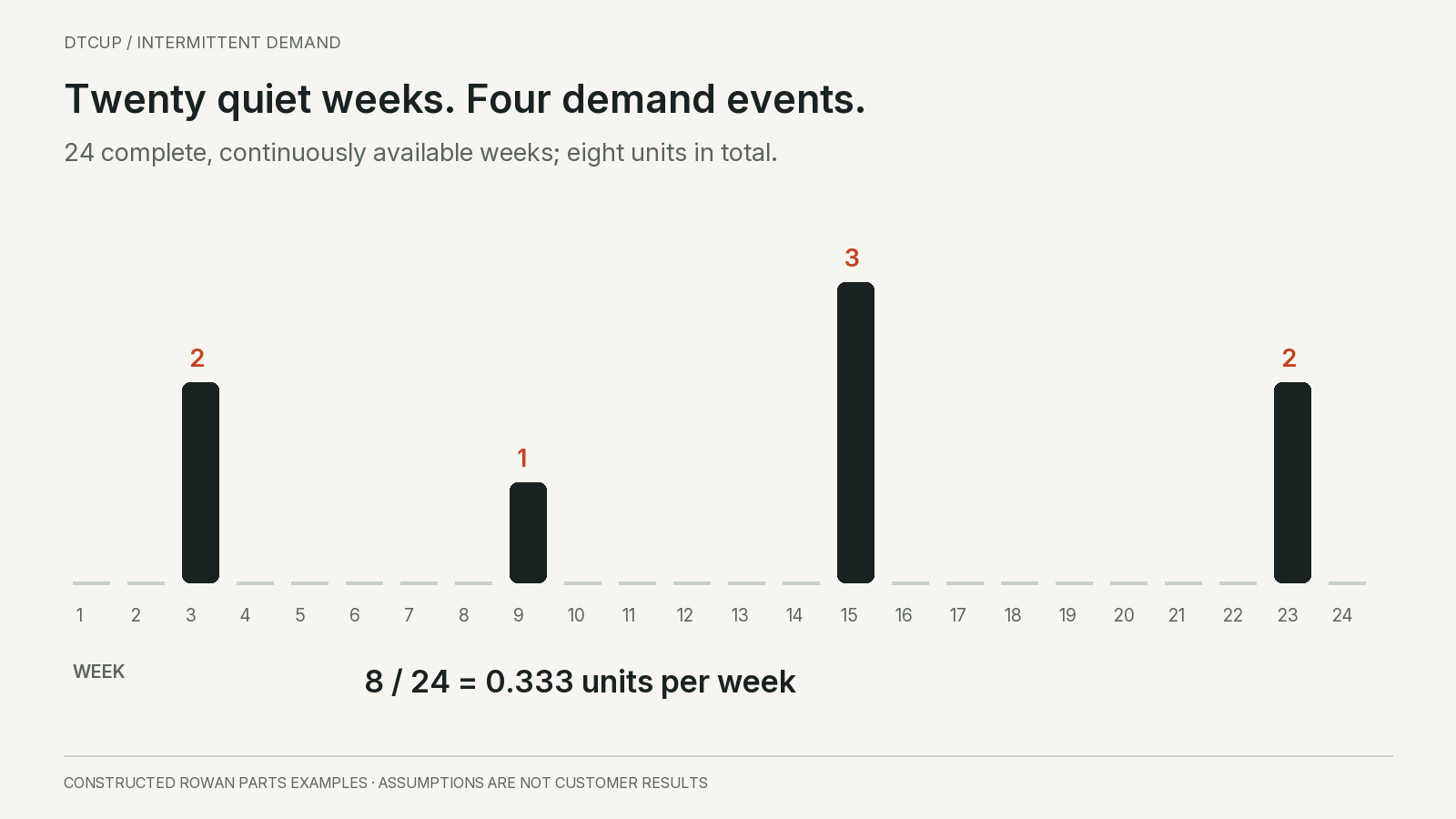
Rowan Parts sells a replacement latch. Across 24 complete weeks, observed eligible demand is positive in only four weeks: two units in week 3, one in week 9, three in week 15 and two in week 23. The other twenty weeks have zero demand. Total demand is eight units, or one third of a unit per week.
That average is a valid summary of the period. It is not a prediction that the warehouse will pick a third of a latch every week. The actual work arrives as discrete requests, separated by long gaps. If the buyer rounds the weekly forecast down to zero before combining periods, the planning system loses the demand entirely.
Look at the pattern at the level where the decision occurs. One latch may sell sporadically in each warehouse but regularly across the network. A product family may sell every week while a specific color or size remains intermittent. A daily history can appear sparse even when weekly replenishment is straightforward. The data interval and location level help create the pattern you see.
Also distinguish low volume from unpredictable size. Some spare parts receive occasional requests for exactly one unit. Another item receives occasional orders for twenty or fifty units. Both have quiet periods, but the inventory consequence of an event is very different. Calling both “slow movers” is not enough to choose a replenishment rule.
Do not infer seasonality from a few visible gaps. Four events cannot establish a dependable annual pattern, and a six-week interval between two pairs of events does not prove that the next order is scheduled. The history may support a rough rate and a range of plausible outcomes while leaving exact timing highly uncertain.
The useful first deliverable is a compact profile: observation period, available selling time, positive periods, units per positive period, longest quiet stretch, current commercial status and replenishment lead time. That profile tells the buyer what is known before a forecast method adds a precise-looking number.
2. Ask whether each zero was observable demand
A zero is meaningful only when the business knows what could have been observed. If the item was available, discoverable and orderable throughout the week, zero eligible orders is an observed zero. If it was unavailable or its listing was hidden, zero orders may reflect constrained access. If the source failed to import, the value is unknown.
Those conditions should not be merged into one cell merely because the forecasting library expects a number. A product that was unavailable for ten of the twenty quiet weeks has a different history from one that customers could buy throughout. The data must preserve that distinction even if the chosen estimation method later handles it through a simplified assumption.
Check whether backorders capture otherwise hidden demand. If customers can place a valid backorder, the order date may record the request despite a stockout. If the checkout blocks the purchase, orders alone cannot reveal how many people wanted the item. A waiting-list signup is another signal with a different meaning, not automatically an order unit.
For Rowan Parts, assume the 24 weeks are complete and the latch was continuously available. This assumption makes the arithmetic clear. In real work, verify it. The stockout demand guide explains how to keep observed and estimated demand separate when availability is incomplete.
Inspect event types as well. A warranty replacement, internal transfer and retail order may all remove units from stock, but they can have different drivers. A service part may need separate forecasts for paid demand and approved replacements before the warehouse combines them into a total requirement. Excluding one stream accidentally can be worse than choosing an imperfect forecasting method.
Returns require similar care. A returned unit is not negative customer interest, and it may not become sellable immediately. Forecast the defined demand stream, then model recoverable supply separately. Otherwise one return in a quiet month can make a small-demand series look negative and confuse both the rate estimate and the purchasing decision.
3. Separate how often from how much
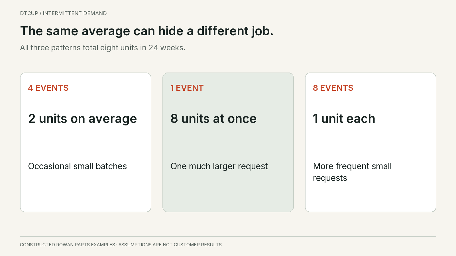
For the constructed latch history, four of 24 weeks contain demand. The observed occurrence frequency is therefore 4 divided by 24, or about 16.7% of weeks. Conditional on a positive week, the average quantity is eight units divided by four events, or two units. Multiplying those summaries gives about 0.333 units per week.
This decomposition does not magically create new information. It reorganizes the same eight units so the buyer can ask better questions. Is the product being requested less frequently? Are positive orders getting larger? Has a new wholesale customer changed event size without changing the number of active weeks? Different answers suggest different planning actions.
Suppose another part has one positive week in the same 24-week period, with eight units in that week. Its overall mean is also 0.333. Yet an eight-unit request is harder to serve from two units on hand than the latch’s typical request. A shared average does not justify a shared stock policy.
A third part might sell one unit in eight different weeks. It has the same total and mean again, but smaller and more frequent events. Depending on replenishment speed and order requirements, it may be easier to support with a small buffer. This is why a portfolio sorted only by average weekly sales can mix very different service risks.
Keep the sample size next to the estimate. Four positive periods provide little evidence about the full range of event sizes. The observed maximum of three is not a guaranteed upper bound. A buyer may need information about installed products, contract customers or replacement compatibility to judge whether larger requests are plausible.
The simple observed frequency is also not automatically a stable future probability. It assumes the historical conditions remain relevant. A discontinued parent product, lost account or changing installed base can alter the process. Treat the two-part summary as a starting description, then investigate what could change each part.
4. Keep simple baselines in the comparison
Begin with a transparent historical-rate baseline. For Rowan Parts, the full-period rate is eight divided by 24. A recent twelve-week rate is five divided by twelve, because weeks 15 and 23 contain three and two units. A recent four-week rate is two divided by four. The estimates are approximately 0.333, 0.417 and 0.5 units per week.
It would be tempting to call those rising values evidence of growth. They could instead be the result of where a short window happens to fall around two events. A single order can change a sparse series sharply. The buyer should inspect the event and its cause before turning a recent-window jump into a permanent increase.
The last observed week’s demand is another possible baseline, but it is often unstable here. It alternates between zero and the size of the latest event. The last positive quantity ignores the waiting time altogether. Neither should be adopted simply because it is easy to calculate; each still provides a useful comparison against more elaborate methods.
A zero forecast is worth including as a diagnostic, particularly when a performance metric rewards quiet weeks. It is not automatically a sensible stock policy. If the evaluation declares zero the winner while the business misses every service request, the scoring method and the operating objective are misaligned.
For each baseline, preserve the information available at the forecast date. A full-history mean calculated after the evaluation period is not an honest forecast for that period. It can explain arithmetic, but it cannot establish predictive performance. Candidate models should be compared using earlier data to predict later periods at the horizon the buyer actually faces.
This prevents a common distraction: spending weeks optimizing an intermittent-demand method without checking whether it improves the purchase decision over a simple rate. The purchase-decision backtesting guide gives the broader evaluation process. Sparse items need that discipline just as much as high-volume sellers.
5. Understand what specialist methods change
Croston’s method separately smooths positive demand quantities and the intervals between them, then forms a rate from their ratio. The classic update occurs when positive demand arrives. It is a useful reference method for intermittent histories, but its output is still an estimated rate rather than a schedule of future orders.
The Forecasting: Principles and Practice discussion of count series notes bias in Croston forecasts and the absence of a standard underlying statistical model from which ordinary analytical prediction intervals follow. Do not attach a normal-looking confidence band to the rate merely because a chart component can draw one. A distribution or simulation needs its own stated assumptions.
Bias-adjusted variants and probability-based methods address different weaknesses. The Teunter–Syntetos–Babai research introduces an approach that updates demand-occurrence probability every period, including quiet periods, while estimating positive demand size. That makes the response to prolonged zeros different from a method whose forecast remains unchanged until another positive event.
The practical buying question is which behavior fits the item and improves evaluated decisions. A part supporting a stable installed base may need a different response to a quiet spell from an accessory for a product being withdrawn. The method name alone cannot tell the system whether demand is temporarily absent or permanently disappearing.
Ask the software provider exactly which variant is implemented, how it is initialized and how parameters are selected. Two systems labeled Croston can use different initial states, smoothing choices or corrections. Reproducing a result requires those details as well as the historical data. A category label in a dropdown is not a complete model specification.
Keep the experiment proportionate to the available evidence. Four positive events cannot support confident tuning of many parameters. A simple method with explicit limits may be more defensible than a complex model selected because it fits those four events closely. Complexity should earn its place in later-period performance and service consequences.
6. Make the response to a quiet stretch explicit
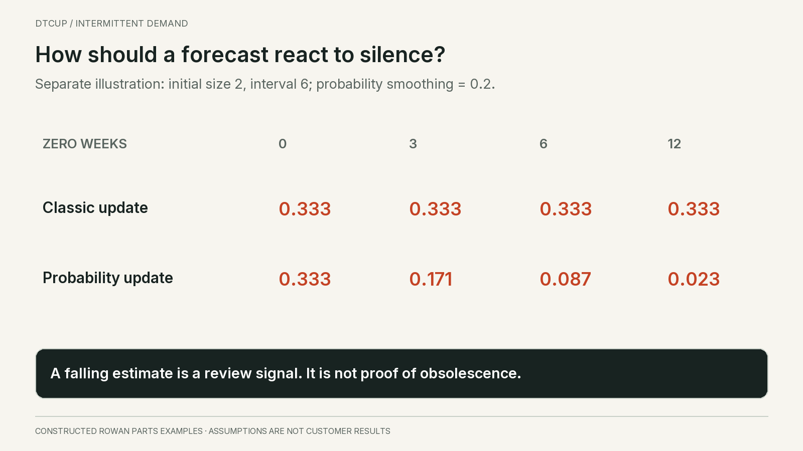
Consider a separate constructed state: the estimated positive quantity is two units and the estimated interval is six weeks. A classic Croston-style rate is therefore two divided by six, or about 0.333 units per week. If no positive event occurs, that rate remains unchanged under the classic update rule.
For a probability-updating illustration, start with an occurrence estimate of one sixth and use a smoothing factor of 0.2. In a zero-demand week, multiply the previous occurrence estimate by 0.8. Keep the positive quantity estimate at two because no new positive quantity has been observed. After three zeros, the rate is about 0.171; after six, 0.087; after twelve, 0.023 units per week.
This arithmetic shows the response mechanism, not a fitted forecast for the original latch history. The starting state and smoothing factor are chosen for explanation. A faster decay might reduce unwanted stock when demand disappears, but it could also underprepare the business for a legitimate order after a normal long gap.
The key operating question is what the quiet period means. Was the parent product discontinued? Did the company lose the account that generated most orders? Has a compatible replacement become the standard? Did the listing stop working? These signals have different implications, and the forecast should not be asked to discover all of them from zeros alone.
A technical decline signal should trigger a review, not automatically erase a service obligation. Rowan Parts may still owe support to an installed base even when purchases become rare. A part with low expected volume can have high customer importance. The decision could be to hold a small central stock, source on request or publish an accurate longer lead time.
Conversely, historical importance does not justify replenishing indefinitely. If the supported population has disappeared, the supplier requires a large final order and compatible alternatives exist, the buyer needs a deliberate end-of-life decision. Record who owns that decision and what evidence would reopen it. A forecast rate that slowly approaches zero is not a substitute for a commercial policy.
7. Plan for the replenishment horizon, not a fractional week
Suppose Rowan Parts must cover four weeks before replacement stock can become available. Multiplying a weekly mean of one third by four gives expected demand of about 1.33 units. That is useful for understanding the average requirement across repeated comparable periods. It is not a promise that one or two units will be enough in the next period.
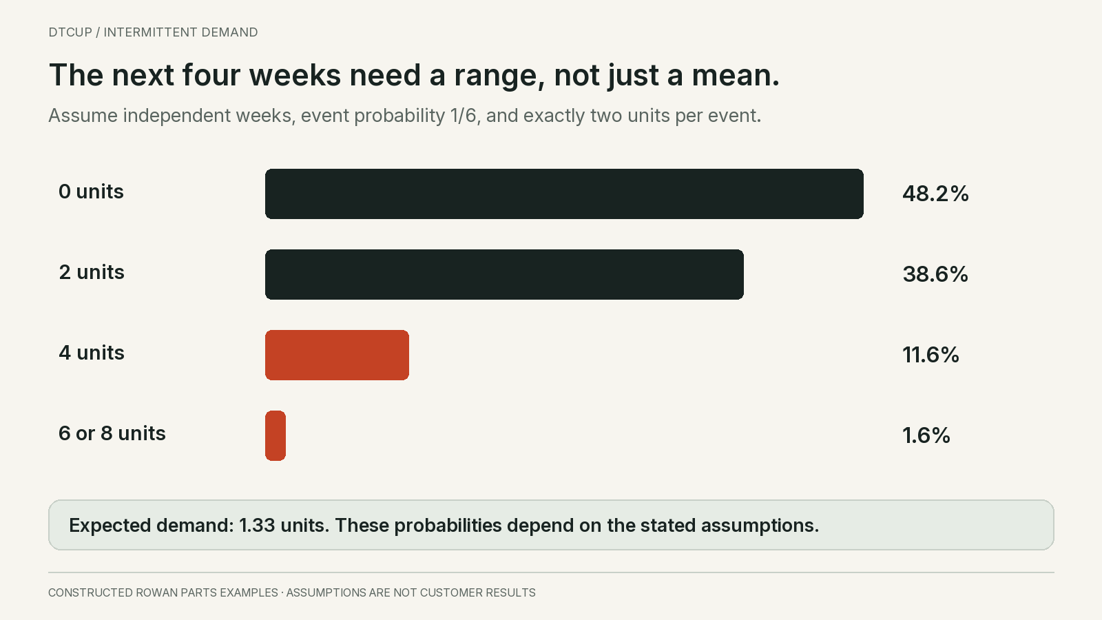
To see the difference, use a deliberately simplified probability scenario. Assume each of the next four weeks independently has a one-sixth chance of a demand event, and every event requires exactly two units. This fixed event size differs from the original observed quantities of one, two and three. The simplification isolates the timing issue; it is not a fitted distribution.
Under those assumptions, the chance of no event in all four weeks is five sixths raised to the fourth power, about 48.2%. The chance of exactly one event is about 38.6%. Two events have probability about 11.6%, while three or four events together account for about 1.6%. Possible total requirements are zero, two, four, six or eight units.
The average remains 1.33 units, but stock of two covers only outcomes with zero or one event: approximately 86.8% of these constructed horizons. Stock of four covers zero, one or two events: approximately 98.4%. These are scenario probabilities of covering the whole horizon, not promised real-world service levels or the fraction of units filled.
The result depends heavily on the assumptions. Demand events might be correlated, a customer might order more than two units, and replenishment might take longer than four weeks. Each could make the simple scenario understate risk. A small history also leaves uncertainty about the one-sixth occurrence estimate itself.
This is why I would show the buyer the rate, the plausible event sizes and the replenishment horizon together. Rounding the mean to one unit conceals the fact that even one event needs two in this scenario. Rounding it to two does not establish an acceptable service level. The stock decision needs the business’s service objective and the consequences of waiting.
Keep pipeline timing visible. Four units on purchase order arriving in week five do not cover a request in week two. Stock reserved for another order may not be available for the next customer. A probability model for demand cannot repair an inventory position that treats all future supply as immediately usable.
8. Aggregate carefully without hiding the customer’s wait
Combining periods can make sparse data easier to inspect. In the original 24-week history, four consecutive six-week blocks contain two, one, three and two units. None of the blocks is zero. The same data now looks much smoother, but the transformation did not create more customer events.
The timing inside each block still matters. A three-unit request at the beginning of a block requires stock earlier than one at the end. If the replenishment decision is weekly, a six-week forecast needs a defensible way to translate back into dated requirements. Dividing evenly may be convenient without representing how orders actually arrive.
Choose aggregation around the decision horizon and inspect its consequences. A monthly service-parts review may benefit from monthly totals. A next-day customer promise still depends on available units when the order arrives. The model can operate at one time scale while the inventory simulation checks another, provided that translation is explicit.
Product aggregation has a similar tradeoff. Forecasting a family may stabilize the estimate, but allocating it to a rare size using last month’s share can produce arbitrary swings. Consider whether the family members share demand drivers and whether the allocation uses enough evidence. A stable total does not prove accurate mix.
Centralizing stock can sometimes reduce the number of locations that each need a buffer, but only if transfer or shipping time meets the service promise. Do not assume that inventory in a distant warehouse is equivalent to local availability. Transport cost, cutoffs, compatibility and customer urgency belong in that decision.
Where history is especially thin, related-item evidence can inform a scenario. Document why the items are comparable: shared installed base, similar replacement mechanism or a common customer contract. Avoid pooling merely because two products have the same color or price. Explain which estimate comes from the item itself and which comes from a broader group.
9. Do not let an accuracy score reward missing every order
Use the original 24-week history for a retrospective scoring illustration. A zero prediction in every week has total absolute error of eight units, because it misses every positive observation. Its mean absolute error is eight divided by 24, or about 0.333 units per week. It looks numerically small because twenty weeks are exactly zero.
A constant prediction of one third in every week incurs about 6.667 units of absolute error across the twenty zero weeks. Across the four positive weeks, the absolute errors also total about 6.667. Total absolute error is approximately 13.333, giving mean absolute error about 0.556. The rate estimate loses this particular comparison even though it acknowledges nonzero demand.
This is not an out-of-sample model test: the rate uses the same history being scored. Its purpose is to expose the scoring behavior. Under absolute error, predicting zero can be attractive when zero is the most common outcome. That does not answer whether a buyer should keep stock for the occasional request.
Nor does this imply that any nonzero forecast is better. Excess stock has a cost, and a declining item may appropriately move toward zero. The evaluation needs to connect predicted demand to a feasible ordering policy and then inspect missed units, waiting time, inventory exposure and any explicit service constraints.
Keep method evaluation and policy evaluation distinct. Two methods can produce slightly different rates that lead to the same order quantity after pack-size rounding. Another small rate change can cross a reorder threshold and produce a large purchase. The business consequence comes from that translation, not from the forecast decimal alone.
The forecast accuracy guide explains denominators, zeros and aggregation in more depth. For intermittent items, I would report the number of positive events alongside any score and always examine what the chosen policy did when those events occurred.
10. Choose a service policy before choosing a buffer
Rowan Parts has several legitimate options. It can hold local stock for immediate dispatch, keep a small central pool, order from the supplier when a customer asks, or retire the item with an approved alternative. The correct choice depends on the promise, the item’s importance, supply reliability and the consequences of a delay.
A replacement latch that makes an expensive product usable again may justify a different policy from a decorative accessory with the same sales history. Revenue ranking alone can miss that distinction. The buyer needs to understand the service role, not simply the last twelve months of sales.
Write the customer promise in operational terms. Does the business need to ship immediately, dispatch within a stated period, or provide a reliable quotation before accepting the order? These promises create different stock requirements. A make-to-order option is only credible if the supplier’s lead time and communication process can support the stated experience.
Then evaluate feasible quantities. If the supplier sells packs of ten, a statistical target of three units is not a purchase order. Existing sellable stock, reservations, confirmed inbound and minimum order rules determine what the buyer can actually do. The forecast should inform the comparison, not bypass it.
For a rare item, the best intervention may be a supplier agreement rather than a more elaborate forecast: smaller packs, shared stock, a dependable expedited route or a substitute approved for the same use. These options change the cost of uncertainty. They can be valuable even when the demand estimate itself barely improves.
Do not describe a policy as optimal without specifying the objective and constraints. Minimizing carrying cost, maximizing immediate availability and preserving support for an installed base can pull in different directions. The decision record should show the chosen tradeoff and who approved it, especially when a low-volume item consumes disproportionate cash.
A final-order decision shows why the service consequence matters
Consider a separate, deliberately simplified final-order scenario for a different Rowan Parts item. There is no opening inventory and no later replenishment during the planning horizon. The team assigns scenario probabilities of 50% to no demand, 35% to two units and 15% to six units. These are planning assumptions, not probabilities estimated from the latch history or a confidence interval.
Expected demand is zero times 0.50, plus two times 0.35, plus six times 0.15: 1.6 units. The supplier permits purchases of two, four or six units at an assumed acquisition cost of $20 each. Unused units have no residual value at the end of this simplified horizon. That last assumption makes this a final-buy example rather than a routine replenishment calculation.
Buying two leaves four units unmet in the six-unit scenario, producing expected unmet demand of 0.15 times four, or 0.6 units. Buying four leaves two unmet in that scenario, or 0.3 expected units. Buying six covers all three stated scenarios. The expected-demand figure alone does not describe those differences.
Suppose the business initially assigns an illustrative $80 consequence to each unmet unit. Combining acquisition expenditure with that penalty gives $40 plus $48, or $88, for a two-unit purchase; $80 plus $24, or $104, for four; and $120 for six. Under these assumptions, two has the lowest modeled total among the three feasible choices.
Now change only the assumed unmet-unit consequence to $200. The totals become $160, $140 and $120. Six becomes the lowest modeled choice. No demand forecast changed. The decision changed because the business valued an unserved request differently. This is why a forecast cannot silently decide the service tradeoff.
The penalty is an analytical device, not necessarily a cash payment. It might represent replacement expense, an approved service remedy or a deliberately weighted customer consequence. It should not be presented as observed lost profit without evidence. If a contractual or safety-related obligation sets a minimum service requirement, treat that as a constraint rather than assuming a convenient penalty can override it.
The scenario also excludes many real complications: uncertain lead time, multiple demand sizes, substitution, salvage value, order handling and information that arrives later. Its recommendation is conditional, not universal. A buyer should change the assumptions to match the actual item and see whether the decision remains stable. A result that flips under plausible assumptions deserves more investigation.
This final-buy framing can be useful when a supplier announces discontinuation. First confirm that the deadline and available quantity are real. Then estimate the supported population, remaining service period and acceptable alternatives. Preserve the evidence behind any scenario probabilities. A confident-looking distribution supplied by an algorithm is not enough when the business is making an irreversible purchase.
For a regular replenishment item, use a multi-period inventory simulation instead. Leftover units may serve later demand, orders can be revised and supplier lead times recur. Counting all leftovers as worthless in that setting would distort the decision. Match the economic model to the actual choice before debating whether the forecast should be 1.4 or 1.6 units.
I would present the buyer with the feasible options and the assumption that most changes their ranking. In this example it is the consequence of an unmet request. In another case it may be remaining support life or salvage value. That identifies the next useful investigation and prevents the team from spending all its effort on a tiny improvement in average forecast error.
Keep the arithmetic reproducible in the purchase record. List the three demand outcomes, their weights, the feasible quantities and the unmet amount for every quantity-outcome pair. A reviewer should be able to replace one assumption without rebuilding the analysis. When the horizon ends, compare the observed outcome with the original scenarios and record what was learned. One realized outcome cannot prove that its assigned probability was correct, but a series of comparable decisions can reveal consistently optimistic or pessimistic assumptions.
11. Evaluate enough complete replenishment cycles
A four-week evaluation with no orders cannot tell you much about how a policy handles intermittent demand. It can reveal excess stock and operating problems, but it contains no positive event to test service. Extend the review across enough relevant cycles and keep the number of observed events visible.
Use rolling forecast dates that resemble the real review schedule. At each date, fit or update the candidate using only information already available. Generate the relevant horizon, apply the actual ordering constraints, and advance through the later demand and receipts. Keep the same initial inventory assumptions when comparing policies.
Separate model selection from final evaluation where the available history allows it. If the team tunes parameters until one unusual order is predicted well and then reports that same period as proof, the result overstates what is known. Sparse data makes this temptation particularly strong because a single event can dominate the comparison.
Where individual items lack enough events, inspect a relevant portfolio as well as item-level exceptions. The portfolio can reveal broad behavior, but it must not hide critical failures. A method that works well for inexpensive accessories may still be inappropriate for service-critical parts. Grouping should preserve meaningful differences in event size, supply and business role.
The Babai, Syntetos and Teunter empirical study examines intermittent-demand methods and the sensitivity of forecasting and stock-control performance to smoothing choices in military and automotive data. Its context is a reminder to evaluate parameters and operating consequences rather than copy a method ranking into a different business. It does not establish a universal winner for a brand’s accessory catalog.
Report uncertainty in the decision. If two policies perform similarly across a small number of events, the honest result may be that neither has demonstrated a dependable advantage. Choose a manageable policy, monitor the next events and avoid an expensive implementation justified by noise. A clear inconclusive result is more useful than an overconfident leaderboard.
12. Use a review card that changes what the buyer does
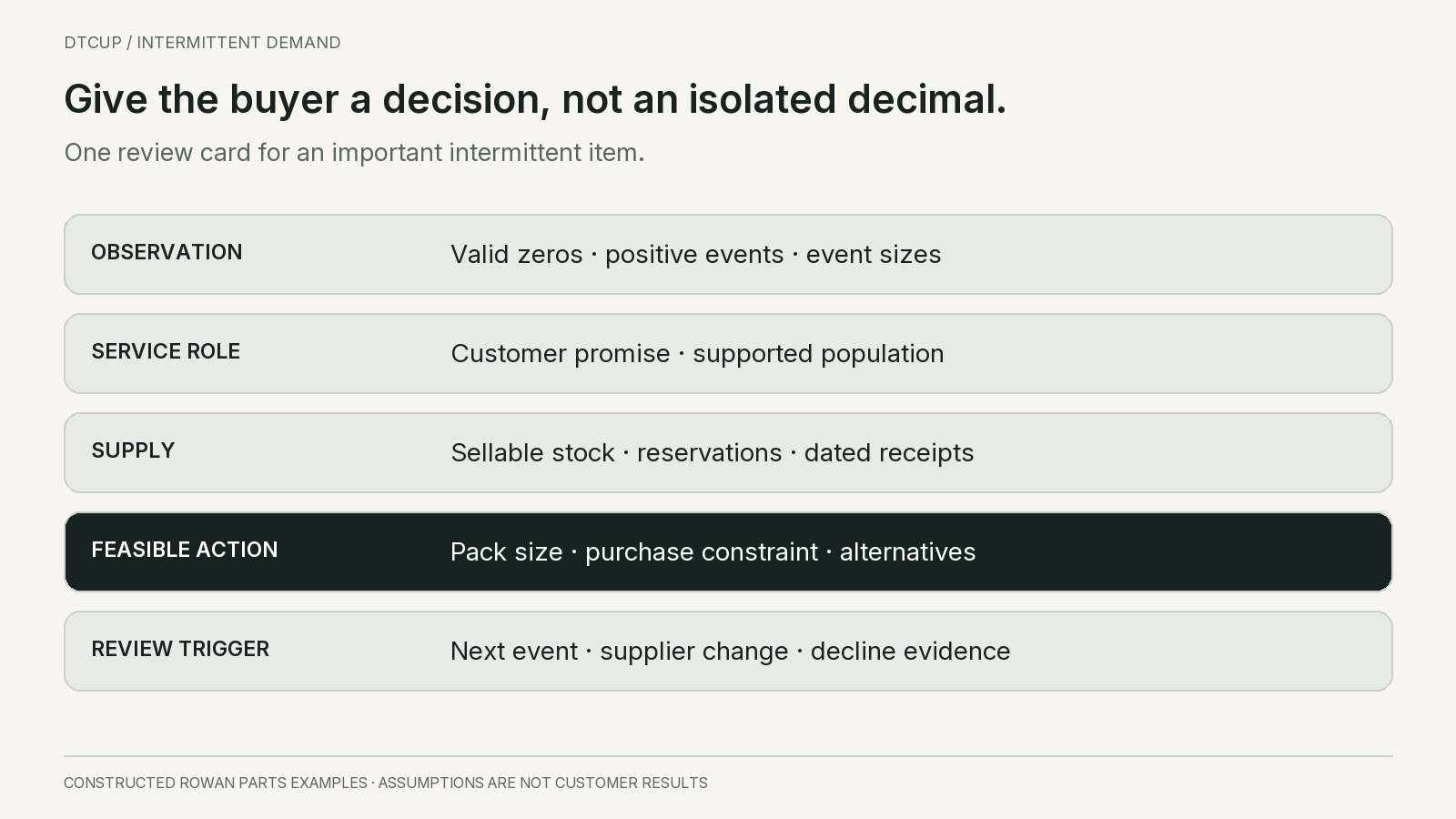
For each important intermittent item, I would maintain one review card. It starts with the item and service role, the demand definition, coverage and availability evidence. Then it shows the positive-event count, event-size summary, current occurrence estimate and any known commercial change. This keeps the number connected to the business.
The next part records supply reality: sellable units, existing commitments, dated inbound, lead-time uncertainty and purchase constraints. A forecast without those fields cannot establish whether the business is exposed. A stock figure without the demand profile cannot explain why the exposure matters.
Finally, record the decision in plain language. For example: “Keep the current central buffer while validating the remaining installed base; do not place the supplier’s ten-unit minimum automatically; review after the next demand event or the supplier’s final-order notice.” This is a fictional illustration, not a recommendation for the latch without further evidence.
Give the review a trigger that matches the risk. A positive event may reveal a larger order size. A prolonged quiet period may justify a decline review. A supplier discontinuation notice may require an immediate final-order decision. A calendar reminder alone is insufficient when important information can arrive between meetings.
Keep overrides separate from the statistical estimate. If the buyer adds stock because a service contract begins next month, record the contract-based adjustment and its expiry. Do not rewrite historical demand to make the model appear to have predicted the event. Future reviewers need to distinguish the forecast, the judgment and the final purchase.
Known future requirements deserve their own line. A confirmed maintenance appointment or accepted customer order is different from an uncertain future request. Decide how the forecast is consumed by those commitments so the same units are not counted twice. For example, the planning record can distinguish firm orders inside the horizon from the remaining uncommitted demand estimate, using an explicit consumption rule appropriate to the business.
Review that rule when large irregular orders appear. If a one-off wholesale request is both included as a firm requirement and treated as evidence that every future week will be equally busy, the buyer can overreact twice. Preserve the order as a real obligation while investigating whether it changes the recurring demand process. Certainty about one purchase does not establish certainty about the next one.
13. Practical questions about intermittent demand
Is a forecast below one unit a mistake?
No. An expected rate can be fractional even when actual orders are whole units. Preserve that rate through the relevant horizon before applying a stock policy. Rounding every weekly estimate down can erase real demand; rounding every week up can create substantial excess. The ordering decision needs event uncertainty, supply timing and feasible pack quantities.
Should every slow seller use Croston’s method?
No. First establish that the series is genuinely intermittent at the decision interval and that zeros are valid observations. Compare transparent baselines and appropriate specialist methods using later periods and inventory consequences. Decline, changing customer contracts, stockouts or obsolescence may require additional information that no method can infer reliably from a short history alone.
How many quiet weeks prove that demand has stopped?
There is no universal number. It depends on the previous occurrence pattern, observation quality and what changed in the market or installed base. A long gap should prompt investigation at a threshold the business has chosen, not automatically become proof of obsolescence. Keep any service obligations and supplier deadlines in the decision.
Can related products help when there is very little history?
They can inform a scenario if there is a defensible shared demand mechanism. Preserve differences in compatibility, customer base and replenishment conditions. Make the borrowed evidence visible and test the resulting decisions as new observations arrive. Pooling unrelated items merely to produce a stable number can hide the uncertainty rather than reduce it.
The best planning approach for a slow seller is often modest: clean observations, an understandable occurrence-and-size estimate, a clear service promise and a feasible supply response. Use sophisticated methods when they improve that decision. Do not ask the forecast to settle a product’s future, a supplier relationship or a customer commitment without the people who own those choices.
Sources
Still have a question?Ask the DTCUP Community ↗