
Promotion Forecasts Without Double-Counting Growth
A promotion can add demand, move it from another product or bring a later purchase forward. Separate those effects before committing stock or calling a sales spike profitable.

7 years of experience building and operating brand websites, specializing in website development, paid advertising and SEO. Built a brand website from launch to US$10 million in annual sales.
The Short Answer
Freeze the no-promotion baseline, explain new demand separately from switching and early purchases, reconcile related products and later periods, then compare timed supply and contribution under explicit scenarios.
Key takeaways
- A promoted-item spike is not the same as range growth.
- Switched and early purchases need corresponding offsets.
- Discounting baseline purchases can outweigh additional volume.
- Scenarios should change customer-response assumptions, not only totals.
- Supply buffers and targets belong outside the expected demand forecast.
- Review operational accuracy separately from causal promotion lift.

A promotion produces a large spike in orders. Marketing calls it a strong campaign, the buyer raises the next purchase order, and finance notices that contribution has fallen. Two weeks later, sales slow below their usual level. The promotion may have worked exactly as designed, but the team used one visible number to answer several different questions.
A promoted product can sell more because the business found additional demand. It can also sell more because customers chose it instead of another product, or bought today instead of next month. All three mechanisms matter for inventory during the event. Only one necessarily adds units across the whole range and the wider period. Treating them as the same kind of growth is a common route to excess stock and disappointing economics.
My preferred approach is to build a promotion forecast as a set of explicit changes around a baseline. Preserve what would probably happen without the event, state what the event is expected to change, and carry the consequences into related products and later periods. Then translate that demand view into supply and contribution. A single uplift percentage should be the result of this reasoning, not a substitute for it.
This guide uses a fictional brand, Fern Table, with two related products. The figures are simplified teaching assumptions, not a customer case or a claimed industry benchmark. Their purpose is to make the logic visible enough that a buyer, marketer and finance owner can challenge the same plan.
Define the decision before estimating an uplift
Start with what the forecast will change. A buyer may need to reserve stock before an event. Marketing may need to decide whether a discount is worth offering. Operations may need to arrange picking capacity. These decisions share demand information, but they do not have identical objectives. A quantity that protects service during a busy week is not automatically the quantity with the best expected financial result.
Describe the event precisely. Name the eligible products, offer, audience, distribution channels, dates and markets. Record whether the event changes price, placement, advertising support or several things together. If the plan is still changing, label the forecast as conditional on the current plan. An estimate for a small customer email should not silently become the forecast for a broad paid campaign.
Set a horizon long enough to include the likely consequences. The event itself may last a few days, while customer purchasing shifts across several weeks. Related products can lose sales during the event, and the promoted product can experience a quieter period afterward. The appropriate review horizon depends on the category and buying cycle; there is no universal number of weeks that captures every effect.
Fern Table chooses a two-week promotion window and a two-week follow-up window for its initial exercise. It will also review later observations for evidence that the follow-up period was too short. The forecast covers both Product A, which will be promoted, and Product B, a close alternative. That scope prevents the team from declaring success based only on Product A’s event-period orders.
Separate the commercial objective from the forecast. The business may want to acquire customers, clear aging stock or support a launch. Those objectives can justify different choices, but they should not alter the estimate merely to make the target appear achievable. A target of five hundred units is not evidence that five hundred units will be demanded.
Write the decision in one sentence. For this example: should Fern Table run the proposed offer, and how much usable Product A stock must be available before the event under low, base and high demand scenarios? This gives the forecast a practical purpose and keeps later analysis from becoming a general debate about whether promotions are good or bad.
Preserve the no-promotion baseline
The baseline is the demand expected without the proposed event, under the other conditions you have specified. It should reflect relevant seasonality, distribution and current business conditions. It is not simply last week’s sales copied forward, and it should not already contain the same promotion effect you intend to add later.
Inspect how the existing forecast was produced. If a model uses a promotion calendar or price features, its output may already include part of the event’s expected effect. If it was trained on promotional sales without distinguishing them, the baseline may also contain historical promotional behavior. Adding a separate uplift without checking this can count the same effect twice.
Keep a visible baseline version before making adjustments. Record its date, included information and known limitations. When someone later proposes an increase, ask what new information is absent from that baseline. “We feel optimistic” is different from “the confirmed distribution plan reaches an additional eligible audience not included in the current forecast.”
Forecasting: Principles and Practice discusses judgmental adjustments as useful when they incorporate important additional information, while warning against unsupported adjustments and recommending documentation. The practical lesson here is to make every override explain what it adds. Do not treat manual involvement as evidence that a forecast has become better.
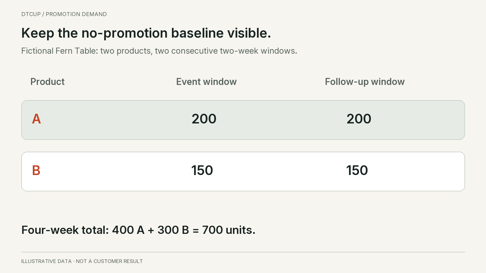
Fern Table’s illustrative baseline is two hundred Product A units in the event window and two hundred in the follow-up window. Product B’s baseline is one hundred fifty units in each window. The four-week total is therefore four hundred A units plus three hundred B units, or seven hundred units across the two-product range.
These are demand assumptions, not a promise that supply will be available. The baseline has not yet been capped by inventory. Keeping demand separate from the sales plan allows the team to see a shortage rather than hiding it inside a lower forecast. The stockout demand guide explains why observed sales can understate the demand a forecast is trying to represent.
Split the promoted product’s increase into different mechanisms
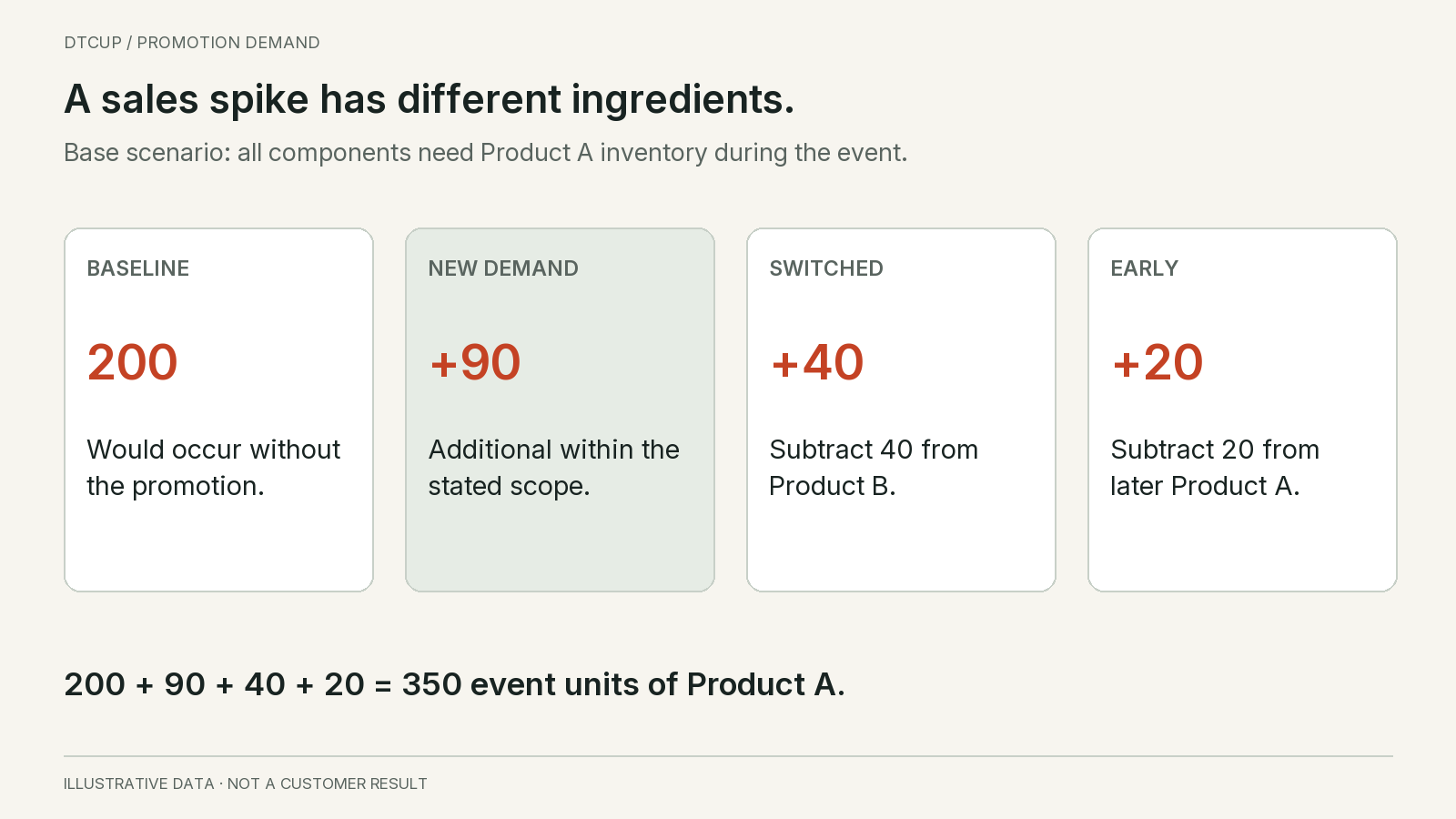
In the base scenario, Fern Table expects Product A to gain one hundred fifty units during the promotion. Instead of entering a single seventy-five percent uplift, the team explains the increase through three assumptions: ninety units of genuinely additional demand within the defined range and horizon, forty units switched from Product B, and twenty units purchased earlier than they otherwise would have been.
The ninety additional units represent demand that would not have occurred in the no-promotion scenario within the chosen scope. This is a forecast assumption, not a measured causal result. It might later be informed by a suitable experiment or stronger historical evidence. Calling it incremental in the planning model does not prove that the real event will create that effect.
The forty switched units are cannibalization within Fern Table’s range. Customers who would have bought B choose A instead. Product A still needs inventory for those orders. But the business should reduce B’s expected demand by the same forty units in this simplified one-for-one substitution example. Leaving B unchanged would invent forty additional range units.
The twenty early units are purchases pulled forward from A’s follow-up window. They increase the event’s stock requirement and reduce later demand. If the buyer uses the event spike to raise the following month’s replenishment without accounting for this shift, the team may buy more just as customers need less.
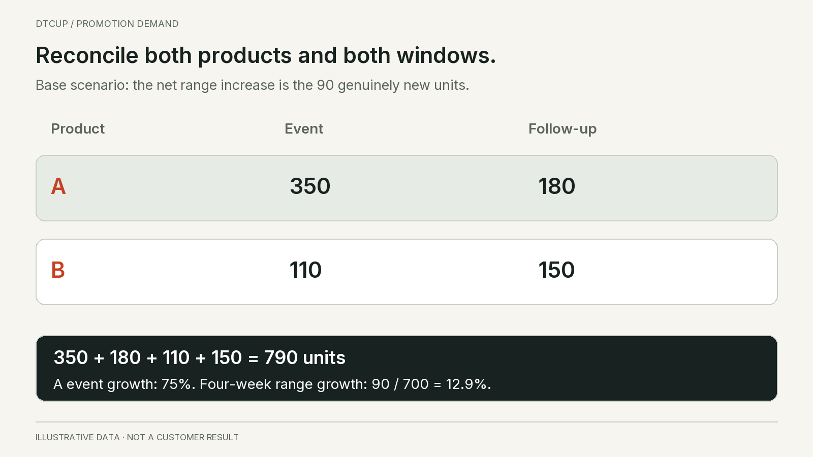
Product A’s event demand becomes three hundred fifty units: the two hundred baseline plus ninety new, forty switched and twenty early. Its follow-up demand falls to one hundred eighty. Product B’s event demand falls to one hundred ten, while its follow-up demand remains one hundred fifty. Every adjustment has a corresponding place in the plan.
The mechanisms can be more complicated in a real assortment. A bundle may contain different quantities, and substitution may not be one for one. Some purchases may shift between channels rather than products. The principle remains the same: state the unit conversion and the scope, then account for the offset wherever it belongs. Do not add all favorable movements while forgetting the corresponding reductions.
Reconcile the forecast across products and time
The completed base scenario contains three hundred fifty A units during the event, one hundred eighty A units afterward, one hundred ten B units during the event and one hundred fifty B units afterward. The total is seven hundred ninety units. Compared with the seven hundred-unit baseline, the range gains ninety units, exactly matching the assumed genuinely additional demand.
Product A’s event-period increase is seventy-five percent. The range’s four-week increase is about twelve point nine percent. Both calculations are correct, but they answer different questions. The first describes the peak requirement for the promoted item. The second describes the net quantity change across the defined products and period. Neither should replace the other.
This reconciliation is a useful error check. If the total increase exceeds the genuinely additional component, look for a missing offset, duplicated adjustment or inconsistent unit definition. If it is lower, inspect whether a reduction has been counted twice or whether the scenario includes another effect that has not been explained.
Preserve both views in the planning meeting. Warehouse operations need to prepare for the concentrated event volume. Procurement needs to understand the later slowdown and the reduced B requirement. Finance needs the complete range and time view. A single aggregate total would hide the peak, while a single promoted-item chart would hide the offsets.
Be clear about the boundary of the ninety-unit conclusion. The example includes only A and B and four weeks. If another product is affected or demand is shifted from a later period, the range and horizon need to expand. A neatly reconciled table can still be incomplete if its scope excludes the place where the offset actually occurs.
Do not use reconciliation as a claim of causal proof. It verifies that the assumptions are internally consistent. It does not verify that the assumptions describe customer behavior. That distinction is important: a coherent forecast is a better planning tool than an incoherent one, but it still needs evidence and later evaluation.
Connect the unit forecast to contribution
More units do not automatically create more contribution. Fern Table assumes that a regular A unit contributes eighteen dollars after the variable costs included in this exercise, before the event’s additional campaign expense. During the promotion, A contributes twelve dollars per unit. B contributes fourteen dollars. The event also requires eight hundred dollars of additional campaign expense.
The no-promotion baseline contributes eleven thousand four hundred dollars: four hundred A units at eighteen dollars, plus three hundred B units at fourteen dollars. The promotion base scenario contributes four thousand two hundred dollars from event A units, three thousand two hundred forty from later A units, and three thousand six hundred forty from all B units. That is eleven thousand eighty before the additional campaign expense.
After the eight hundred-dollar expense, contribution is ten thousand two hundred eighty dollars. It is one thousand one hundred twenty dollars below the no-promotion baseline. This is a decision-scope contribution comparison, not a complete accounting profit statement. Fixed overhead and effects outside the stated scope are excluded, and the unit contribution assumptions already include the relevant variable costs.
The result can also be explained by mechanism. The ninety genuinely additional A units add one thousand eighty dollars at the promotional contribution. The forty switched units lose eighty dollars because each replaces a fourteen-dollar B contribution with a twelve-dollar A contribution. The twenty early units lose one hundred twenty dollars because they replace later eighteen-dollar A contributions with twelve-dollar contributions now.
The two hundred baseline A units also receive the discount, losing six dollars each, or one thousand two hundred dollars. Combining these effects gives a three hundred twenty-dollar reduction before campaign expense. Subtract the additional eight hundred and the difference is again negative one thousand one hundred twenty. This second calculation is a useful check on the first.
The example does not prove that promotions are unprofitable. It shows why the composition of the uplift matters. A plan that acquires many genuinely additional purchases can produce a different result from one that mostly discounts existing demand. The pricing architecture guide explains the wider offer and margin context; this calculation connects that context to the forecasted units.
Build scenarios by changing mechanisms, not just percentages
A low, base and high forecast should describe plausible differences in behavior. Multiplying the same total by an arbitrary percentage creates a range, but it does not tell the team what would make the range occur. Change the underlying assumptions so that each scenario has an operational explanation.
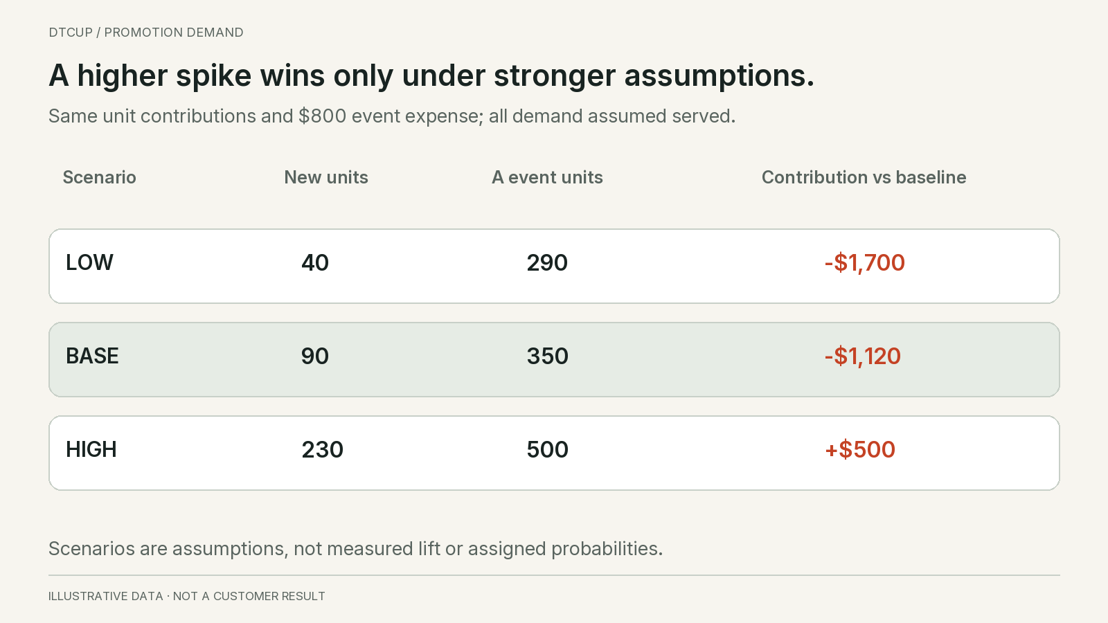
Fern Table’s low scenario contains forty new units, thirty switched units and twenty early units. Product A therefore needs two hundred ninety units during the event and one hundred eighty afterward. B needs one hundred twenty during the event and one hundred fifty afterward. The range total is seven hundred forty units, and contribution after the same campaign expense is nine thousand seven hundred dollars.
The base scenario remains ninety new, forty switched and twenty early units. It requires three hundred fifty event A units, totals seven hundred ninety range units, and produces ten thousand two hundred eighty dollars of contribution after campaign expense. Its loss against the baseline is one thousand one hundred twenty dollars.
The high scenario assumes two hundred thirty new units, forty switched units and thirty early units. A needs five hundred units during the event and one hundred seventy afterward. B remains at one hundred ten during the event and one hundred fifty afterward. Total range demand is nine hundred thirty units. Contribution after campaign expense is eleven thousand nine hundred dollars, five hundred dollars above the baseline.
The high case reverses the commercial conclusion because genuinely additional demand is much larger. That is the assumption the team must defend, not just the impressive headline of five hundred event units. What evidence supports reaching that many additional buyers? How similar is the audience to previous events? Can the website and fulfillment operation serve the demand?
Do not attach probabilities unless you have a defensible basis for them. It is acceptable to use unweighted scenarios to expose consequences. An invented probability distribution can make an unsupported forecast appear precise. If probabilities are used, document their source and test how sensitive the purchase or promotion decision is to them.
Find the commercial hurdle behind the sales target
The mechanism view lets Fern Table calculate a useful hurdle. Hold the base assumptions of forty switched units and twenty early units fixed. The discount on two hundred baseline A units costs one thousand two hundred dollars of contribution. Switching costs eighty, early purchasing costs one hundred twenty, and the additional campaign expense is eight hundred. Together, those effects create a two thousand two hundred-dollar contribution hurdle.
Each genuinely additional promotional A unit contributes twelve dollars under the stated assumptions. Dividing the hurdle by twelve gives about one hundred eighty-three point three units. Since the example plans whole units, it needs at least one hundred eighty-four genuinely additional units to exceed the no-promotion contribution. Ninety new units in the base case are well below that hurdle.
This is more informative than a target of four hundred sales. With one hundred eighty-four new units, forty switched units, twenty early units and two hundred baseline units, event A demand would be four hundred forty-four. A target of four hundred event units could still miss the contribution hurdle even if the team achieved it. Total event sales do not reveal their composition.
The hurdle is conditional, not a universal break-even rule for this product. If the discount changes, both the contribution on new units and the loss on baseline units change. If campaign expense rises to reach a larger audience, the hurdle rises too. If switching is toward a higher-contribution product rather than away from one, the economics change again. Recalculate the complete comparison instead of carrying the original threshold into a different offer.
Use this calculation to challenge the plan constructively. The team could test a smaller discount, reduce avoidable event costs or target an audience less likely to buy at full price anyway. Each alternative needs its own response assumption; a smaller discount may also attract fewer new buyers. The point is to identify the commercial condition that must be true, then design a credible way to test it.
Do not assume future repeat purchases will close the gap. They may contribute value, but that requires evidence about additional customers, later behavior and the costs of serving them. Keep a near-term contribution result and a separately labeled future-value scenario. Otherwise an unmeasured lifetime-value claim can make any promotion appear profitable.
Translate demand into a timed supply plan
A demand scenario is not yet a purchase order. The buyer must compare it with usable stock, existing reservations, confirmed receipts and the time required to replenish. A large quantity arriving after the promotion does not protect service during the event. Keep the dates and availability states visible.
Suppose Fern Table has three hundred twenty usable A units available for the promotion and cannot receive more until after it ends. The base demand scenario is three hundred fifty, so there is a thirty-unit shortfall. The high scenario has a much larger shortfall. Do not lower the demand forecast to three hundred twenty and then report that the plan is fully covered.
Instead, maintain separate lines for unconstrained demand, available supply and the feasible sales plan. The sales plan may be capped at three hundred twenty under the stated assumptions, while the demand view preserves the expected unmet portion. The team can then decide whether to bring stock forward, narrow the offer, change the event date or accept the shortage.
Do not assume which demand component is lost when stock runs out. The unserved customers might have been new buyers, buyers switching from B or customers purchasing early. That composition affects the financial result and later demand. A simple supply cap does not tell you how to revise the contribution calculation without another assumption.
Break the event into time periods appropriate to the operational risk. A two-week total may conceal a first-day spike. Use the actual email schedule, advertising plan and historical event shape where relevant. But do not invent daily precision when only a rough total is supported. A small number of timing scenarios can be more useful than a smooth daily curve with no evidence.
The inbound inventory guide helps distinguish promised receipts from usable supply. Combine that discipline with the promotion forecast. The campaign should not rely on an optimistic receipt date that nobody in operations has accepted.
Check the purchase constraint after calculating the need. A supplier’s pack size or minimum order can force a larger commitment than the event requires. Put the resulting leftover exposure into the supply decision, including the quieter follow-up period. Do not reinterpret the extra purchased units as additional forecast demand. The MOQ and pack-size comparison shows how a lower unit cost can still create a less attractive cash and inventory outcome.
Agree contingencies before launch pressure arrives
A forecast range is useful only if the team knows what to do when reality moves toward one end. Decide before launch which signals justify a change and who can approve it. For Fern Table, that might mean reviewing accepted orders and usable inventory at a defined cadence, with a separate check on whether the advertising and email plan was delivered as intended.
Do not react to an early spike without considering the event’s shape. A launch email may concentrate expected demand in the first hours. Conversely, a slow start may reflect a delayed send rather than weak customer response. Compare actual performance with the planned timing and confirmed execution before changing a purchase order or adding another discount.
Set practical limits for any response. If supply is running short, an approved option may be to reduce promotion exposure or explain a later delivery date accurately. If demand is weak, the team may pause additional paid support rather than extending the discount automatically. Every response changes the original scenario, so record the decision and preserve the first forecast for review.
Protect the customer promise when the plan changes. Do not continue advertising an availability or delivery claim that operations cannot support. Coordinate the landing page, offer configuration, customer service guidance and campaign materials. A promotion forecast is connected to those promises because it determines the workload and stock behind them. The most useful contingency is one the team can execute coherently across the customer journey.
Avoid stacking the same growth in several places
Double-counting often enters through collaboration rather than a formula error. Marketing adds expected campaign lift. Sales adds a seasonal increase. Procurement adds a safety allowance. Management adds a stretch target. The resulting number may look like consensus even though several adjustments describe the same demand or serve different purposes.
Use an adjustment register with the original baseline, the proposed change, the reason, the owner and the affected period. Require the proposer to identify what information the baseline lacks. If a seasonal effect is already modeled, it should not be added again merely because the event occurs in a strong month.
Separate demand adjustments from supply protection. Safety stock is a policy response to uncertainty and service objectives. It is not additional expected customer demand. If the buyer adds a buffer, show it in the supply decision rather than increasing the forecast and then applying another buffer to the inflated forecast.
Separate planned distribution from hoped-for performance. A confirmed increase in advertising exposure can inform a scenario, but it does not guarantee a proportional order increase. Audience saturation, conversion differences and overlap with existing customers can change the response. Explain the conversion assumptions rather than multiplying spend growth directly into demand.
Watch for overlapping audiences across channels. The same customer may receive an email and see an advertisement. Adding independent channel forecasts can count the same likely purchase twice. Use a combined event view and state how overlap is handled. Where the evidence is weak, represent that uncertainty in the scenario instead of pretending the channel estimates are additive.
A forecast meeting should end with one approved demand view and a visible record of disagreements or scenario alternatives. It should not erase the baseline or the reasons for overrides. The judgmental forecasting principles in Forecasting: Principles and Practice distinguish forecasts from targets and supply decisions. Keeping those roles separate makes the meeting more useful.
Learn from comparable events without copying their uplift
Historical promotions can provide evidence, but “last time we sold twice as much” is not yet a transferable estimate. Compare the offer, product maturity, audience, distribution, availability, season and competitor context. A launch event supported by a large new audience may not resemble a routine discount sent to existing customers.
Record whether the historical event was supply constrained. If stock sold out, observed sales are a lower bound on demand under those conditions, not a complete measure of response. If the website failed or the offer was misconfigured, the event may be a poor basis for estimating the intended promotion. Preserve those defects in the event record rather than treating the result as a clean observation.
Compare the pre-event baseline and the follow-up period. A large spike followed by a dip suggests a question about timing, but it does not prove pull-forward by itself. Seasonality, competing activity or a stock problem could also explain the pattern. Use the evidence to build and challenge assumptions rather than assigning a causal label from the chart’s shape alone.
For a new event, choose a small set of relevant analogs and explain the adjustments. A less dramatic but more comparable campaign can be a better guide than the largest event in the archive. Avoid selecting only the best historical results. The buyer needs a realistic range, not a highlight reel.
Keep the unit of comparison consistent. A percentage increase from a tiny baseline can look extraordinary while adding few units. A promotion of a multipack can change selling units without changing underlying component demand in the same way. Translate pack and bundle quantities before comparing events.
The short-history forecasting guide explains how to use analogs without inventing seasonality. Promotion planning benefits from the same restraint: state which historical evidence transfers, which does not, and what information would make the next forecast more reliable.
Separate forecast review from causal evaluation
After the event, compare the observed outcome with the forecast, but do not assume the difference from baseline is the promotion’s causal effect. The baseline is an estimate of what would have happened without the event. Other conditions may have changed at the same time. A forecast review and an incrementality study answer related but distinct questions.
The forecast review asks whether the plan helped the business prepare. Did stock arrive before the peak? Were the right products available? Did the event shape match the timing assumptions? Did the follow-up period contain excess stock? These questions can produce useful operational improvements even when the causal lift remains uncertain.
A causal evaluation asks what the event changed relative to an appropriate alternative. Depending on the setting, that may require a controlled test or another defensible design. It also needs to account for the affected range and time horizon. Measuring only the promoted product during the discount period can miss substitution and early purchasing.
Do not judge a stock-constrained forecast only by realized sales. If the plan called for three hundred fifty units but supply allowed only three hundred twenty, the observed shortfall is not automatically a demand forecasting error. Record the constraint and use the available evidence to assess unmet demand cautiously. Otherwise the next forecast can learn that the shortage was normal demand.
Likewise, a commercially poor promotion can be forecast accurately. Fern Table’s base scenario could occur almost exactly as predicted and still reduce contribution. Forecast accuracy tells you whether the expected response was understood; it does not tell you whether choosing the offer was wise. Keep those judgments separate in the review.
The incrementality decision guide is useful when the team needs stronger evidence of additional sales. Use it alongside the inventory review, rather than asking either discipline to answer every question about the event.
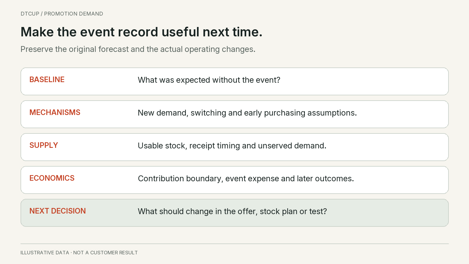
Write an event record the next planner can use
Capture the plan before launch and the outcome afterward in the same record. Include the offer, audience, dates, prices, baseline, adjustment assumptions, scenarios, supply constraints and decision owner. Preserve the original forecast rather than replacing it with the actual result after the event. Otherwise the team loses the evidence needed to learn.
Record changes during the event. A campaign may be extended, an email may be delayed, an item may sell out, or a discount may be corrected. These changes can explain a forecast miss. They should not become excuses invented after the fact; retain the timing and the actual operational evidence.
Review the promoted item, related items and the follow-up period together. Include contribution on the agreed cost boundary, not only revenue or unit growth. If later returns change the result, update the review with a clear cutoff date. The first event recap may be useful for operations while the commercial result is still maturing.
Translate the review into a specific rule for next time. Perhaps the event needs a narrower audience, a smaller discount, a later date or an earlier stock commitment. Perhaps the baseline already captured seasonality and the manual adjustment was unnecessary. A useful lesson changes a future decision; “the campaign was strong” does not.
Keep uncertainty in the record. If the team cannot separate new demand from switching with the available data, say so. The next event can be designed to improve that evidence. An honest limitation is more useful than a precise decomposition written after the outcome to make the plan appear correct.
A compact event library becomes valuable over time because it preserves comparable conditions and decisions. It does not need a complicated model at the beginning. It needs consistent definitions, reliable records and a team willing to inspect where its assumptions were wrong.
Questions to resolve before approving the promotion
Should the forecast include the sales target?
Show the target beside the forecast, not inside it. The gap can reveal how much additional demand the plan would need to create. Management may choose a more ambitious campaign or accept a different supply risk, but that decision should not erase the estimate. A forecast that is edited until it matches the target cannot provide an independent reality check.
Is cannibalization always bad?
No. A customer may move to a product that serves them better or creates more contribution. A business may intentionally simplify its range or introduce a new item. The issue is whether the shift is understood and included in the comparison. Count the offset and evaluate the full economics instead of treating every promoted-item increase as additional business.
How far after the event should we look?
Choose a horizon related to the buying cycle and the decision, then check whether important effects continue beyond it. A frequently purchased consumable may show timing shifts differently from an infrequent durable purchase. The four-week example is a teaching boundary, not a universal recommendation. If the result changes materially when the horizon extends, explain that sensitivity.
Should we stock for the high scenario?
Not automatically. Compare the cost of excess stock, the consequence of shortages, replenishment flexibility, cash limits and the confidence in the scenarios. The demand forecast describes possible needs; the inventory policy chooses how much risk to carry. Keep that choice explicit and avoid disguising a service buffer as expected demand.
Can an application calculate the answer for us?
An application can organize eligible order history, forecasts and scenario inputs, but it cannot make unsupported assumptions true. Verify which promotion features and data sources are actually available in the product you use. DTCUP Demand should be evaluated on its connected data and current capabilities; this guide does not claim that every decomposition or campaign simulation shown here is an automated product feature.
Approve the whole plan, not just the spike
A good promotion forecast explains the shape of the business change. It shows what would happen without the event, what is expected to be genuinely additional, what moves from another product and what moves from a later period. It also shows when stock must be usable and what the offer does to contribution.
For Fern Table, the base case needs substantially more Product A stock during the event even though the total range grows modestly and contribution falls. The high case can justify a different conclusion, but only if its much larger new-demand assumption is credible and supply can support it. That is the discussion worth having before the purchase order and campaign are approved.
Keep the baseline, adjustments, supply policy and target separate. Reconcile across products and time. Then use the event review to improve the next decision. This is how promotion planning becomes a repeatable commercial discipline instead of a recurring cycle of excitement, shortages and unexplained leftover stock.
Sources
Still have a question?Ask the DTCUP Community ↗