
Forecast Accuracy: WAPE, Bias and the SKUs an Average Can Hide
A forecast can balance in total and still leave the wrong stock on the shelf. Work through error direction, volume weighting, zero demand and scaled comparisons before trusting one accuracy percentage.

7 years of experience building and operating brand websites, specializing in website development, paid advertising and SEO. Built a brand website from launch to US$10 million in annual sales.
The Short Answer
Preserve forecast vintage, horizon and demand basis, then calculate signed and absolute errors at the decision level before aggregation. Read WAPE with its volume denominator, inspect SKU bias and zero-demand cases, compare a same-horizon baseline and connect consequential misses to the inventory policy.
Key takeaways
- Zero total bias can hide offsetting SKU errors.
- Calculate absolute errors before combining products or periods.
- WAPE measures error relative to volume, not the probability of being correct.
- Keep zero, missing and stockout-constrained demand distinct.
- Scaled scores need a meaningful training reference and a direct future baseline comparison.
- Weighting error by value does not turn it into realized financial loss.

A forecast can be exactly right for the total business and wrong for every product the buyer needs to order. One SKU is short by a hundred units, another is long by a hundred, and the overall variance is zero. The dashboard looks balanced. The warehouse contains the wrong stock.
This is why I would not approve a demand forecast from one accuracy percentage. A useful review separates the size of errors, their direction, the level at which they are calculated and the operating consequence. WAPE, bias, MAE and scaled errors can all help, but each answers a narrower question than “Can we trust this replenishment plan?”
The examples in this guide use a fictional business, Cove Supply, and deliberately small constructed datasets. Every forecast, quantity and cost is illustrative. None is a claim about a real model or customer result. The arithmetic is simple enough to reproduce in a worksheet so the reader can see exactly where a reassuring average becomes misleading.
The goal is a practical forecast review: a consistent error ledger, a small set of complementary measures and an exception list that tells the buyer where to investigate. This guide focuses on interpreting the measures. The separate purchase-decision backtesting guide explains how to connect a forecast comparison to a simulated buying policy.
1. Freeze what the forecast was actually trying to predict
Before calculating an error, write the forecast contract. Identify the product, location, demand definition, time bucket, forecast creation time and future period being predicted. “May demand for item C100, issued before May began” is different from an estimate revised during the final week of May. Both may be useful, but they must not compete as if they had the same information.
Preserve forecast vintages. A forecast vintage is simply the version issued at a particular decision time. If a system overwrites last month’s forecast with today’s improved estimate, its historical report can look accurate for the wrong reason. The buyer needs to know whether the information available when the purchase was placed was good enough.
Match the horizon to the decision. A next-week forecast may support warehouse staffing, while a forecast across the next eight weeks may support an overseas purchase. A model that performs well one week ahead can perform poorly at the replenishment horizon. Report the horizons separately rather than mixing them into an average that has no clear user.
Define actual demand carefully. Ordered units, shipped units and units remaining after refunds are different quantities. Cove’s worked examples use nonnegative eligible order units, with cancellations and exclusions resolved under a documented rule. They do not silently subtract returns into negative demand. If the business predicts net revenue instead, it needs a different unit and interpretation.
Availability matters. Observed sales during a stockout do not reveal all demand that might have occurred. A forecast can appear to overpredict when the item simply could not be bought. Keep constrained periods identifiable and assess them separately. Any estimated lost demand should remain distinguishable from observed orders, as explained in the stockout demand guide.
Finally, specify the evaluation population. Are discontinued items included? Are new launches assessed separately? Are only active locations counted? Changing these rules can move the score without changing the forecast. Publish the coverage count and exclusions beside the metric so the team knows which decisions the result supports.
This contract may look like administrative work, but it prevents the most expensive comparison errors. A precisely calculated score is still misleading if it compares different demand definitions, different information dates or different populations. Fix those boundaries before debating which formula is best.
2. Start with signed error and absolute error
Use one sign convention throughout the report. In this guide, signed error equals forecast minus actual demand. A positive number means overforecasting; a negative number means underforecasting. Some software uses the opposite convention. Neither is inherently wrong, but an unlabeled sign can reverse the meaning of the management discussion.
Absolute error removes the sign and keeps the size of the miss. If actual demand is 100 units and the forecast is 80, signed error is minus 20 and absolute error is 20. If the forecast is 120, signed error is plus 20 and absolute error is still 20. Direction and magnitude are separate observations.
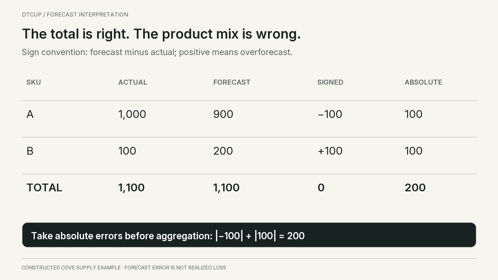
Cove’s first example has two SKUs. Item A has actual demand of 1,000 and a forecast of 900. Item B has actual demand of 100 and a forecast of 200. Item A is underforecast by 100; item B is overforecast by 100. The total actual demand and total forecast are both 1,100.
The summed signed error is zero, but summed absolute error is 200 units. Those numbers do not contradict each other. The first says that overforecasting and underforecasting balance at the total level. The second says that the item-level plan misses by a combined 200 units. A buyer cannot usually replace an unavailable A with surplus B simply because the arithmetic balances.
Store both columns in the underlying ledger. Add absolute error only after matching each forecast to its corresponding actual. If the system aggregates forecasts and actuals first, then takes the absolute difference, it produces zero in this example and erases the item mismatch.
Also preserve the number of observations. Mean absolute error, or MAE, is total absolute error divided by the count of evaluated observations. Across these two item observations, MAE is 100 units. That is easy to interpret, but the unit size and observation definition matter. An average across single items, cartons and kilograms would not be meaningful without a deliberate common basis.
The ledger is more valuable than the summary alone because it allows the business to change the question without reconstructing history. An analyst can inspect directional bias, a buyer can inspect missed units by SKU, and a manager can inspect financial exposure. They should all be able to trace their view back to the same matched records.
3. Read WAPE together with its denominator
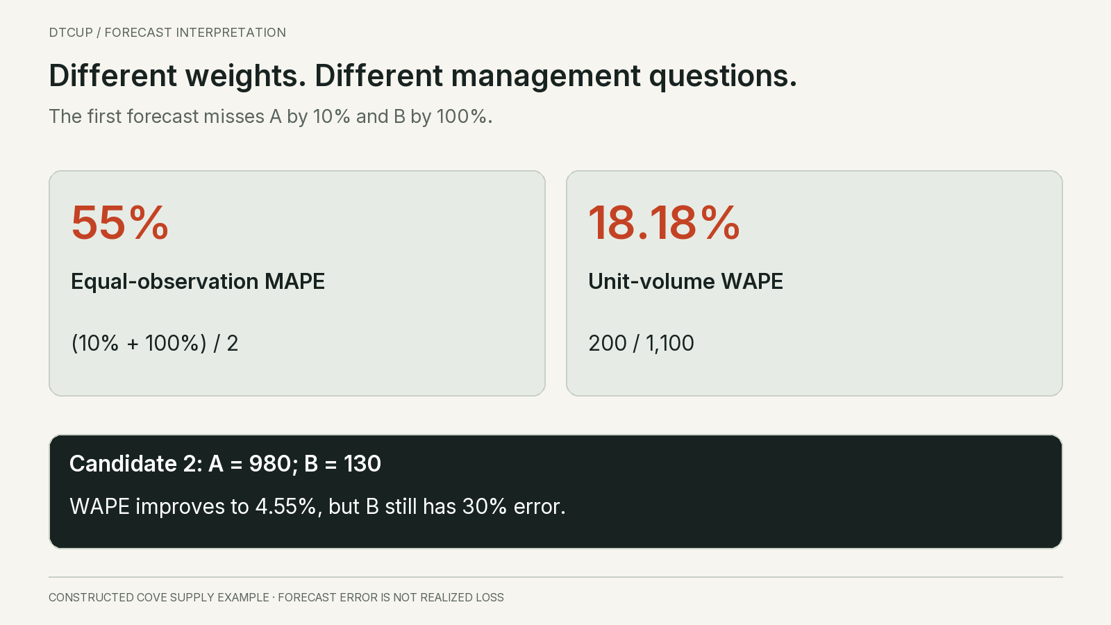
For the nonnegative unit-demand examples here, weighted absolute percentage error, or WAPE, is the sum of item-level absolute errors divided by the sum of actual units, multiplied by 100. Cove’s two-SKU example gives 200 divided by 1,100, or approximately 18.18%. The numerator must retain the item-level misses before it is summed.
WAPE can be useful as a compact measure of absolute error relative to the evaluated volume. It gives larger-volume observations more influence than an unweighted average of individual percentage errors. That weighting can be appropriate for a capacity discussion. It can also hide an important failure in a low-volume, high-value or strategically important item.
Do not describe 100 minus WAPE as a universal probability of a correct forecast. An 18.18% WAPE does not mean that 81.82% of SKUs were correct, that 81.82% of customers were served or that the buyer has an 81.82% chance of avoiding a shortage. Those are different quantities requiring different observations.
WAPE can exceed 100%. That is mathematically possible when total absolute error is greater than the actual volume. Clipping the score to make an “accuracy” gauge look tidy hides information. Display the error measure directly and explain the cause rather than forcing every result into a zero-to-one-hundred success scale.
Watch for denominator growth. Suppose the absolute error is ten units when actual demand is 100, producing 10% WAPE. Later, the same ten-unit error occurs when demand is 200, producing 5%. The percentage improved because the actual volume doubled. The absolute miss did not change. Whether that is operationally better depends on the decision, not the percentage alone.
Rob Hyndman’s discussion of WAPE highlights limitations when the evaluation denominator changes with the series, including trending data, and the undefined result when all evaluated actuals are zero. That is a reason to treat WAPE as one scoped diagnostic, not a universally comparable measure across changing periods.
Keep the absolute-error numerator, actual-volume denominator and evaluated row count beside the percentage. These three numbers make it easier to spot a changing population or scale. If the report only exposes the final percentage, a team can spend weeks explaining a supposed model improvement that was actually a different sales mix.
For regular reviews, compare the same item population and horizon where possible, then show additions and removals separately. A portfolio WAPE can still be useful, but it should sit above item or segment diagnostics rather than replacing them. The summary tells you where to look; it does not tell you what to buy.
4. Use bias to detect direction, not to certify accuracy
In this guide, normalized bias is summed signed error divided by summed actual demand. The sign follows forecast minus actual. A positive value indicates net overforecasting; a negative value indicates net underforecasting. The same zero-denominator issue applies when actual volume is zero, so show the signed unit error separately.
Cove’s two-SKU portfolio has zero normalized bias because minus 100 and plus 100 cancel. Item A nevertheless has a minus 10% bias and item B a plus 100% bias for this single evaluated observation. The portfolio is directionally balanced and operationally mismatched at the same time.
Persistent direction is more useful than an isolated sign. One underforecast can be ordinary uncertainty. A sequence of underforecasts in the same product family may indicate an omitted promotion, a stale growth assumption or a systematic difference between the demand definition used for training and the one used for purchasing.
Plot signed errors over time rather than relying only on their sum. Alternating large positive and negative misses can average near zero. A long run of small negative misses may produce a modest overall score but repeatedly leave the buyer short. These patterns suggest different repairs and different buffer needs.
Do not automatically correct every observed bias by multiplying next month’s forecast. First inspect whether the cause is likely to persist. An isolated launch, a late data import or a one-time bulk order can distort a short window. A mechanical correction may turn yesterday’s exception into tomorrow’s systematic overforecast.
Separate the statistical demand forecast from the stocking decision. A buyer may intentionally stock above a central demand estimate to protect a service commitment. That does not mean the underlying forecast should be inflated until it no longer represents its stated target. Keep the forecast, safety allowance and order constraints as separate fields so their purposes remain visible.
When reviewing overrides, compare the original forecast and adjusted forecast against the same later actuals. Preserve who changed the value, when and why. An override that fixes a known promotion is different from one added because a manager dislikes a low number. Without a reason record, the operation cannot learn which human adjustments help.
Bias is a diagnostic invitation: where are we repeatedly leaning in the wrong direction, and what mechanism explains it? It is not a score that should be forced to zero at every level. A balanced total can still contain serious item-level errors, while a deliberate service decision may rationally hold more stock than average demand.
Ask which statistical target the forecast represents. A mean estimate, a median estimate and an upper demand quantile are not interchangeable promises. An upper quantile is intended to sit above many realized outcomes, so evaluating its signed error as if it were an unbiased mean can produce the wrong criticism. Record the target and use an evaluation appropriate to it rather than silently relabeling every forecast as expected demand.
If the system supplies a range, retain its endpoints and stated coverage separately from the central value. Check how often actual demand falls inside the range over comparable cases and whether the range is useful for planning. A very wide range can cover many outcomes while offering little purchasing guidance. Central-value error, range coverage and decision usefulness deserve separate judgments.
5. Compare item-level and portfolio-level views
An unweighted mean absolute percentage error, or MAPE, gives each nonzero evaluated observation equal weight after expressing its error as a percentage of actual demand. In Cove’s first example, item A’s absolute percentage error is 10% and item B’s is 100%. Their average is 55%, compared with the 18.18% WAPE.
The measures differ because they weight the observations differently. Neither calculation is a clerical mistake. MAPE gives the small item the same observation weight as the large item. WAPE weights by actual unit volume in this nonnegative example. The correct interpretation depends on whether the decision concerns total volume, typical item behavior or a particular service exposure.
Now consider a second candidate forecast: 980 for item A and 130 for item B. Absolute errors are 20 and 30, totaling 50. Its portfolio WAPE is approximately 4.55%, and its MAPE is 16%. Both are better than the first candidate on this small constructed dataset.
Even so, item B remains overforecast by 30% while item A is underforecast by 2%. A manager who sees only the 4.55% portfolio result may conclude that every SKU is ready for unattended ordering. The item view shows why that conclusion would be premature. A model can improve materially while still requiring targeted review.
Use segmentation that reflects decisions. High-volume stable items, new launches, intermittent sellers and discontinued products may need different interpretation. Critical spare parts may deserve attention despite low revenue. A small item with a long replenishment lead time can create a larger service problem than a high-volume item that can be replenished tomorrow.
Avoid averaging already-aggregated percentages without their denominators. If one warehouse has 20 units of absolute error on 100 actual units and another has 20 on 900, the combined WAPE is 40 divided by 1,000, or 4%. Averaging 20% and approximately 2.22% would produce approximately 11.11%, a different weighting question.
Neither view needs to disappear. The combined measure describes the pooled unit volume. The equal-warehouse average treats the two warehouses as equally important reporting units. Label which weighting is intended. A report becomes misleading when it changes weights silently while keeping the same metric name.
I would give the buyer both a portfolio summary and an exception list ordered by a clearly stated decision priority. The list might begin with repeated underforecasting in long-lead items, large cash exposure from overforecasting or unusually poor performance in a new launch. That makes the aggregate useful without allowing it to hide the work.
6. Handle zero demand without removing the difficult rows
Percentage errors become awkward when actual demand is zero. Dividing an individual absolute error by zero is undefined. Removing those rows makes the report easier to calculate, but it also removes evidence about overforecasting on quiet periods. For slow sellers, those periods may be most of the history.
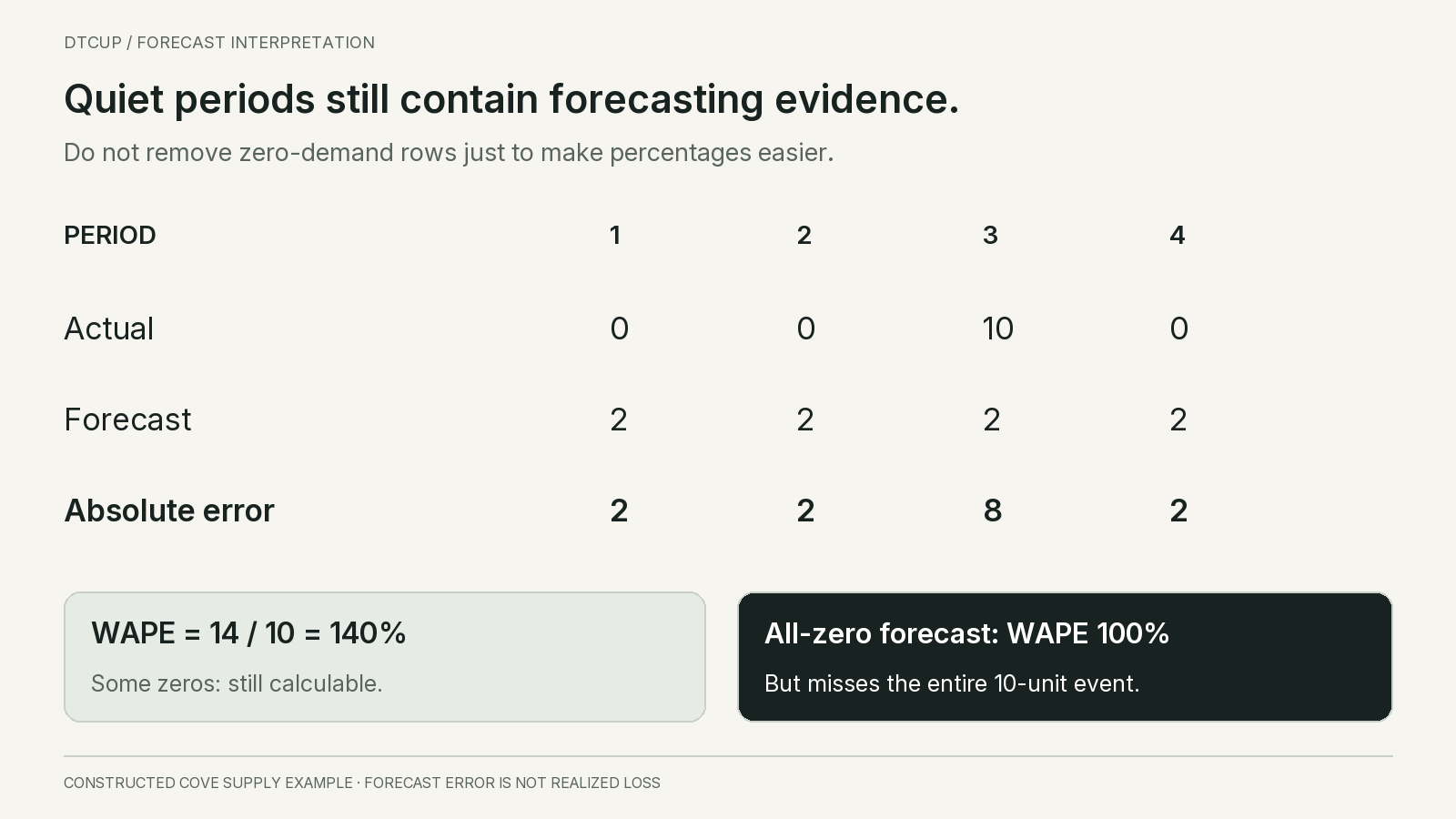
Consider a four-period demand sequence of zero, zero, ten and zero units. A forecast of two units in every period has absolute errors of two, two, eight and two. Total absolute error is fourteen units and total actual demand is ten, so WAPE is 140%. Signed error totals minus two, producing minus 20% normalized bias under this guide’s convention.
Individual MAPE cannot be calculated normally for the three zero-demand periods. A report that retains only the ten-unit period would show 80% error and ignore the six forecast units placed into zero-demand periods. That is not the same population as the WAPE calculation. Explain exclusions rather than presenting the two numbers as directly comparable.
A forecast of zero in every period has total absolute error of ten and WAPE of 100%, better than the two-unit forecast on this particular measure. Yet it misses the entire ten-unit event. If the business needs to keep a critical item available, the lower absolute-error score does not settle the stocking decision.
This example illustrates a mismatch between a point-error objective and a service objective. Sparse demand can reward a low or zero central prediction under some error measures. The stocking policy still needs to consider the consequences of the occasional demand event, supply lead time and the chosen service target. Those decisions should not be hidden inside an “accuracy” ranking.
If every evaluated actual is zero, WAPE is undefined. Show “not defined for an all-zero actual window,” then report the forecast units and absolute error. A forecast of eight units against zero observed units is still useful information. It does not require an invented percentage or a division-by-small-number trick to become visible.
Do not add an arbitrary tiny constant to every denominator and call the result comparable to standard MAPE. The choice of constant can dominate the score for low-volume items. If an operation deliberately uses a modified metric, give it a different name, document the formula and explain why that modification supports the decision.
Keep missing observations separate from observed zeros. A failed order import is not evidence of zero demand. A period before launch is not automatically an active selling period. A stockout zero is constrained information. These data states require different treatment before any forecasting measure is calculated.
For a slow-selling portfolio, review event timing, demand size when it occurs and lead-time demand alongside point errors. A compact error table can still be useful, but it should not force sparse products into the same interpretation as steady daily sellers. The difficult rows are where the operating judgment is most needed.
7. Preserve timing and location before aggregating
Aggregation can hide errors across time as well as across SKUs. Suppose actual weekly demand is ten units followed by ninety, while the forecast is ninety followed by ten. The two-week total is exactly right at 100 units. At the weekly level, absolute errors total 160 and WAPE is 160%.
Which view matters depends on the decision. If all stock can arrive before both weeks and there are no timing constraints, the total may support one purchasing question. If staffing, allocation or replenishment depends on weekly demand, the reversed timing matters. The report should not claim that one aggregation level answers both questions.
The same issue appears across warehouses. Demand can be forecast correctly for the national total while stock is positioned in the wrong region. If transfers take longer than the customer promise, national balance does not prevent local shortages. Evaluate at the location level used by the allocation decision and retain a separate total for broader planning.
Product hierarchies also matter. A family forecast can be accurate while the variant mix is wrong. That may be acceptable when final configuration is flexible, but costly when colors or sizes are manufactured separately. The business should decide where substitution is feasible rather than assuming that errors cancel because items share a category.
Choose the level before reviewing the result. A team can always find a broader aggregation that makes the forecast look smoother. Moving from daily SKU-location rows to monthly category totals after seeing a poor score changes the question. It may produce a useful additional view, but it should not replace the original decision-level evaluation.
For each major use case, keep a named view: purchase-horizon demand by item, weekly demand by location, or monthly family demand for capacity planning. Make the hierarchy and bucket explicit in the title. A metric labeled only “forecast accuracy” invites readers to apply it outside the level where it was calculated.
Reconciliation checks should confirm that lower-level forecasts add to the displayed higher-level forecast when the method is designed that way. If different teams produce separate forecasts at each level, expose the difference rather than silently treating them as one coherent plan. A total that cannot be traced to its components is difficult to act on.
Timing errors also suggest different repairs. A forecast that gets total promotion demand right but shifts it a week late may need a better event calendar. A forecast that consistently gets the size wrong may need different explanatory inputs. Preserving the error pattern helps identify the mechanism instead of merely ranking models.
8. Use a baseline and understand what scaled errors compare
A model can have an impressive-looking percentage while adding little value over a simple forecast. Compare it with a practical baseline issued at the same time for the same horizon. Last observed demand, a seasonal repeat or another transparent operating rule may be appropriate depending on the data. The baseline must use only information available at the forecast date.
Forecasting: Principles and Practice explains the distinction between errors on new observations and residuals from fitted history, and describes scaled measures that use a training-history benchmark. The important operational point is that fitting old data closely is not the same as forecasting future data well.
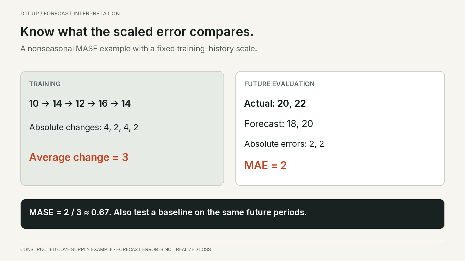
Mean absolute scaled error, or MASE, divides the evaluation-period MAE by a scale calculated from simple differences in the training history. For a nonseasonal example, use the average absolute change from one training observation to the next. The scale is fixed from the recorded training data rather than from the future actual volume being evaluated.
Cove’s small training sequence is ten, fourteen, twelve, sixteen and fourteen. Absolute consecutive changes are four, two, four and two, averaging three. The later actual values are twenty and twenty-two, and the candidate forecasts are eighteen and twenty. Both absolute errors are two, so evaluation MAE is two and MASE is two divided by three, approximately 0.67.
That 0.67 compares the candidate’s evaluation error with the average one-step naive error scale from training. It does not by itself prove that the candidate beat every baseline over the future evaluation horizon. For a direct test, calculate the competing baseline’s actual forecasts over the same held-out periods.
In this constructed example, a fixed-origin last-value baseline predicts fourteen for both future periods. Its errors are six and eight, giving MAE seven. The candidate’s MAE of two is better on these two observations. This direct comparison is easy to understand, but two observations are far too little evidence for a confident production conclusion.
A squared-error version gives larger misses more influence. Root mean squared scaled error, or RMSSE, uses a training scale based on squared changes and an evaluation root mean squared error. Here the training squared changes average ten, while candidate squared errors average four. RMSSE is the square root of four divided by ten, approximately 0.63.
Scaled measures have boundaries too. A constant training sequence can produce a zero scale. Structural breaks or unusual training events can make the historical scale a poor reference for the current task. Seasonal data require a justified seasonal lag, not a convenient choice made after seeing which score looks best.
Use these measures when they improve comparability, and keep their inputs inspectable. A buyer does not need to memorize every formula, but should be able to ask what the score is being compared with. A number without a baseline story is difficult to convert into a purchase decision.
9. Connect errors to economic exposure without calling every miss a loss
Units alone do not express every business consequence. In Cove’s first two-SKU example, suppose item A has a planning value of two dollars per unit and item B fifty dollars per unit. Weighting the absolute errors by those values gives 200 dollars for A and 5,000 dollars for B, or 5,200 dollars of weighted error exposure.
The actual-volume value is 1,000 times two plus 100 times fifty, or 7,000 dollars. A value-weighted absolute-error ratio is therefore approximately 74.29%. That is very different from the 18.18% unit WAPE because the small item carries a much larger value per unit. The weighting changes the question.
Call the result weighted error exposure, not realized loss. Underforecasting does not automatically cause a lost sale if inventory or replenishment absorbs the miss. Overforecasting does not automatically create a write-off if the product sells later. Actual economic consequences depend on the stock position, supply response, substitution, cash timing and aging risk.
Choose the value basis deliberately. Selling price, landed cost and contribution margin represent different concerns. A revenue-weighted measure can prioritize expensive items; a cost-weighted measure can highlight purchasing exposure. Neither is a universal replacement for a service measure. Keep the chosen weights fixed during a comparison or explain the change.
Asymmetry matters. Missing one unit of a critical component may delay a larger order, while holding one extra unit may be inexpensive. For a perishable product, excess can be more damaging. A symmetric absolute-error measure treats equal-sized over- and underforecasts similarly even when the operating consequences are different.
Use a separate scenario or inventory-policy evaluation to represent those consequences. State the shortage and holding assumptions, show sensitivity and avoid presenting a guessed penalty as an audited financial result. This is where forecast evaluation connects to the buying decision, but the connection should remain explicit rather than being hidden inside an unexplained accuracy score.
Cash constraints can also change the priority. A modest error on a high-cost product may tie up capital needed for a reliable seller. A low-cost item may deserve a larger buffer because it protects the availability of a bundle. The exception list should reflect these dependencies instead of sorting solely by the largest percentage error.
Keep at least one unweighted or clearly unit-based view alongside the financial view. Otherwise changing prices can make the model appear better or worse even when its quantity forecasts are unchanged. The purpose of weighting is to clarify a decision, not to manufacture a more favorable ranking.
10. Avoid the leaderboard traps that make models look better
Do not select the metric after seeing which model wins. Decide the main decision-level measure and supporting diagnostics before the comparison. It is reasonable to inspect several measures, but the final recommendation should explain tradeoffs rather than quietly choosing whichever score favors a preferred system.
Use the same evaluation rows for competing forecasts where possible. If one model fails to produce difficult items and the report excludes those rows, its remaining average may look excellent. Show coverage and failures separately. Missing predictions are part of operational reliability, not a convenient way to shrink the test set.
Preserve manual overrides and post-processing. A model output rounded to case packs is no longer the same quantity as an unconstrained demand estimate. Evaluate the raw forecast for forecasting questions and the feasible order for purchasing questions. Blending the two makes it hard to tell whether an error came from prediction, rounding or policy.
Do not repeatedly tune against the final evaluation period and then describe it as untouched evidence. Use development comparisons to choose settings, retain a separate later check where feasible, and report the sequence honestly. A benchmark becomes less informative as it becomes part of the design process.
Watch for overlapping horizons. Weekly forecasts for the next eight weeks share many future observations. Their errors are not independent simply because they occupy different rows. A large row count can overstate the amount of independent evidence. Keep origin and target period in the ledger and avoid casual statistical confidence claims based only on row totals.
Show distribution as well as averages. A median item error, upper-tail error or count of severe misses can reveal whether improvement is broad or concentrated. Define thresholds in units or operating terms where possible. An extreme percentage on one unit of demand may be less urgent than a moderate miss on a constrained high-volume product.
Review stability across relevant periods. A model that wins during ordinary weeks and fails during every promotion may still be useful within a restricted scope. A single global winner is not always necessary. The business can choose a default approach with explicit exceptions, provided ownership and switching rules are understandable.
Finally, separate mathematical improvement from release readiness. Data arrival, forecast coverage, runtime, explanation and recovery behavior matter to the buyer. A small error improvement may not justify a system that misses the ordering deadline or cannot explain why a product suddenly disappears from the plan.
11. Run an accuracy review that changes the plan
Begin the meeting with the evaluation contract and coverage. State the demand basis, forecast vintage, horizon, item-location population and actual-data maturity. Show how many records were excluded and why. This takes little time when the definitions are stable and prevents the meeting from spending half an hour arguing about incompatible numbers.
Next, show absolute error and directional bias at the decision level, then a relative or scaled measure where appropriate. Include the actual-volume denominator. Add a direct comparison with the agreed baseline. This compact set usually provides more insight than a dashboard filled with several differently named percentage scores.
Move quickly to the exceptions. Select a small set that represents different mechanisms: repeated underforecasting, a large overforecast exposure, a zero-demand problem, a timing shift and a data-quality failure. Trace each one to the underlying ledger. The aim is to identify a repair, not to embarrass a planner or defend an algorithm.
For each exception, separate forecast error from supply failure. A correct demand forecast cannot prevent a late supplier receipt by itself. A poor forecast may cause no service failure when enough stock already exists. Keeping those mechanisms separate helps the business assign the right owner and avoid changing the model to compensate for an unrelated operational defect.
Write the action in a form that can be checked later. “Add the confirmed promotion start date to the next forecast vintage” is more useful than “improve seasonality.” “Review the three long-lead items with repeated negative bias” is more actionable than “reduce WAPE.” The metric should lead to a bounded investigation or operating change.
After the next cycle, review whether the mechanism changed as expected. A better portfolio average is not enough if the targeted item remains wrong. Keep the original forecast, adjusted forecast and actual outcome visible. This creates a record of which interventions improve decisions and which merely change the presentation.
The review should end with one of four conclusions for a defined scope: retain the current approach, adjust a specific input or rule, restrict automated use for a problematic segment, or gather better evidence. It does not need to declare a universal winning model every week.
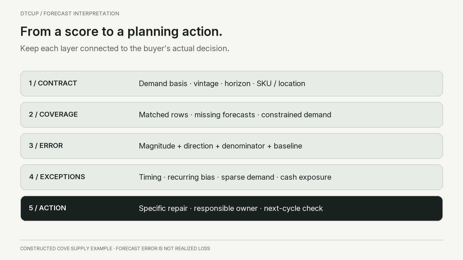
12. Practical questions about forecast accuracy
What is a good WAPE?
There is no universal threshold that proves a forecast is fit for purchasing. Interpret the value against the same population, horizon and demand basis, a credible baseline and the consequences of errors. A threshold chosen for stable high-volume items may be inappropriate for launches or intermittent demand. The buyer’s decision determines what level of error is tolerable.
Can bias be zero while the forecast is poor?
Yes. Equal overforecasts and underforecasts cancel in the signed total. Inspect absolute errors and their distribution across products, locations and periods. Zero net bias says the directions balance at that aggregation level; it does not say the right inventory will be in the right place at the right time.
Should we choose only one metric?
Choose a primary measure for the defined comparison, then keep complementary diagnostics for direction, scale, coverage and operating consequences. More metrics do not automatically create insight. A small set with explicit purposes is easier to use than a leaderboard where every stakeholder selects the number that supports their preferred answer.
Is MASE below one enough to approve a model?
No. It describes performance relative to its training-history scale, subject to that scale being meaningful. Also compare actual candidate and baseline forecasts over the same future periods, inspect consequential misses and check the purchasing outcome. A favorable scaled score is evidence for a decision, not the decision itself.
What should a small team do first?
Save forecast versions, define the actual-demand basis and build a matched item-period ledger with signed and absolute errors. Reconcile totals and inspect a few real exceptions before adding advanced measures. Once the underlying records are trustworthy, a modest report can reveal more than a sophisticated accuracy gauge whose denominator no one understands.
Sources
Still have a question?Ask the DTCUP Community ↗