
Inbound Stock Is Not Available Stock: Plan Around Uncertain ETAs
The same purchase order can produce very different service outcomes. Work through partial receipts, inspection holds and delayed release before deciding whether to transfer stock, expedite or change a promise.

7 years of experience building and operating brand websites, specializing in website development, paid advertising and SEO. Built a brand website from launch to US$10 million in annual sales.
The Short Answer
Model incoming units as conditional supply on the date they become usable. Calculate shortages within complete receipt scenarios before averaging outcomes, preserve partial quantities and release states, and compare contingencies against the specific service gap they can change.
Key takeaways
- Committed, dispatched, received and released quantities have different meanings.
- Identical ending stock can conceal different customer delays.
- Probability-weighted receipts can describe a shipment path that never happens.
- Evaluate scenario consequences before calculating expected cost.
- A transfer changes location stock, not total network stock.
- The last useful action date can precede the official late-receipt date.

A purchase order can show enough units to cover the month while the warehouse runs out next week. The problem is not always the quantity ordered. It is often the way the plan treats an expected receipt as though it were already usable stock.
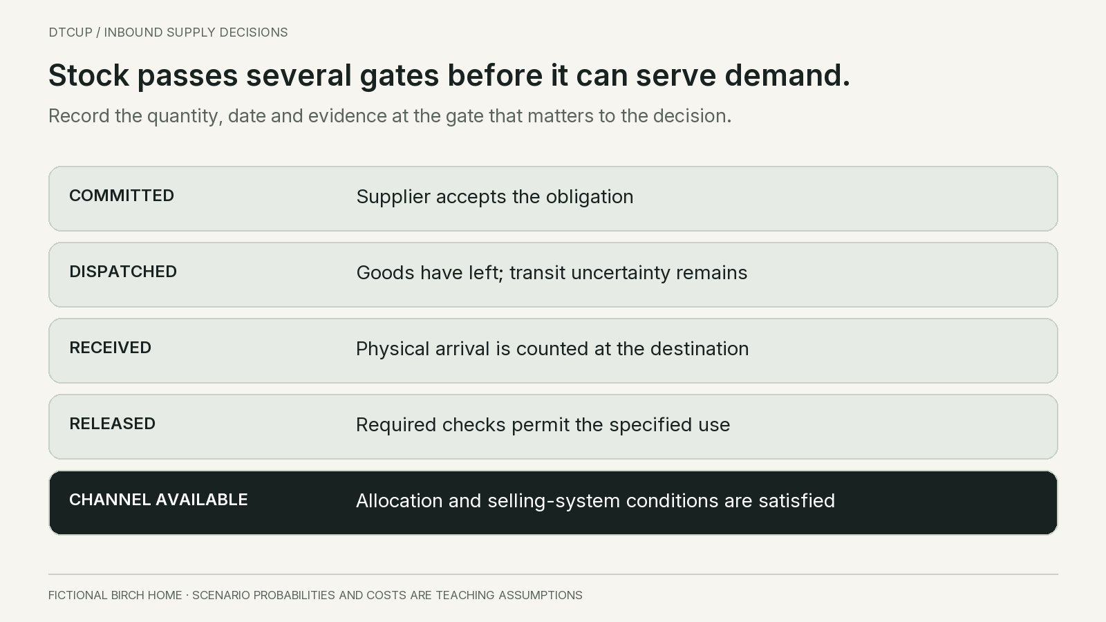
The phrase arriving Tuesday is particularly dangerous because it can mean several things. A vessel reaches a port. A truck reaches a receiving door. A warehouse counts the cartons. Quality approves the batch. The inventory system makes units available to the selling channel. Each event matters, but only some can support the customer promise being made.
I would plan inbound stock as dated, conditional supply. Each expected quantity needs a location, a usable-state definition and evidence supporting its date. Then I would compare several plausible receipt paths against demand and the decisions still available. This makes uncertainty visible without pretending that every late shipment can be predicted precisely.
This guide goes beyond mapping the stages of lead time. It uses a fictional company, Birch Home, to work through partial receipts, delayed release, expected-value traps and contingency economics. All quantities, probabilities and costs are teaching assumptions. They are not supplier benchmarks, forecasts for a real brand or claims about connected DTCUP data.
Name the supply state before counting the units
A drafted purchase order is an intention. An accepted order is a supplier commitment under its stated conditions. Production complete is evidence of progress. Dispatched goods are moving. Received goods are physically at a location. Released goods have met the conditions required for use. Available-to-promise quantities may apply further allocation and channel rules.
Keep these states separate even when a small team uses one spreadsheet. A column named inbound with a single date cannot explain whether the remaining uncertainty is production, transport, inspection or system release. Without that distinction, the buyer may pay for faster freight when the real bottleneck is unfinished production.
State also determines which calculation can include the quantity. A forward planning scenario can include a conditional receipt on a future date. Current sellable stock should not include it as though it were ready now. A customer promise may require a stronger evidence threshold than an internal purchasing scenario.
Quantity needs the same discipline. Two hundred ordered units are not necessarily two hundred inspected units or two hundred units available to the website. Short deliveries, damage, sample use, allocations and pack conversions can change the usable amount. Retain the ordered, received, held and released quantities rather than overwriting them with one convenient number.
Warehouse software reflects this distinction in different ways. Microsoft’s inventory-blocking guidance, for example, describes controls that prevent specified stock from being processed or consumed and distinguishes expected release from present availability. Your own system’s configuration must be verified; an on-hand label alone does not establish that every unit can fulfill an order.
For an internal transfer, include the departure from the source location as well as the receipt at the destination. The transfer moves stock through the network; it does not create new network stock. A destination forecast that adds the receipt while the source forecast ignores the departure can make both warehouses look protected by the same units.
Begin the review by asking what each visible quantity actually allows the business to do. If the answer is only that somebody expects it eventually, keep it in the conditional supply plan rather than silently converting it into current availability.
Build one receipt record that several teams can interpret
The basic planning record should identify the purchase order line, item, unit of measure, destination and expected usable quantity. Add the current milestone, the date being forecast and what that date means. These fields let the buyer and warehouse discuss the same object.
Preserve three versions of an important date: original commitment, current forecast and actual completion when known. If every supplier update replaces the original date, the team loses the evidence needed to evaluate reliability. A shipment can look on time against yesterday’s revised estimate while being weeks late against the commitment that justified a campaign.
Record who supplied the latest update and when. A carrier event, a supplier statement and a planner’s assumption have different evidential value. None is automatically perfect, but the decision owner should be able to see the difference without searching a chain of messages.
Use a usable-at timestamp or a clear daily convention. In the examples here, receipts become usable before demand on the stated day. A real warehouse may have an afternoon release that misses the same-day fulfillment cutoff. If the planning bucket is daily, adopt a conservative documented rule for that case rather than assuming every arrival serves the whole day.
For a split receipt, create child lines whose quantities reconcile to the outstanding parent quantity. Keep the relationship visible. Do not leave the original full receipt active and then add the partial deliveries on top. That mistake produces an attractive forecast from duplicated supply.
Track open quantity after each actual receipt and any approved cancellation. An expected two hundred units followed by an actual eighty-unit receipt leaves one hundred twenty outstanding, unless another documented adjustment changes the order. The first receipt is evidence about part of the order, not confirmation that the remainder will arrive on the same date.
Include an exception owner and the last date an action can still help. A receipt that threatens a launch in ten days may need a decision today if the alternative route takes nine days. The most useful alert is not simply late; it explains the decision window that is closing.
Keep the customer-facing promise in a separate field or process. Internal planners should be able to examine an optimistic scenario without automatically publishing it as a delivery date. The person approving the promise needs to understand the remaining dependencies and the evidence threshold.
Freeze a demand baseline before comparing receipt paths
Birch Home starts a ten-day planning horizon with one hundred eighty sellable, uncommitted units at the destination warehouse. The example assumes demand of thirty units every day. There are no additional reservations, returns, losses or other receipts unless explicitly added.
Total demand is therefore three hundred units. One purchase order has two hundred forty units outstanding. If all demand eventually waits and is fulfilled, the ending balance after the full receipt is one hundred twenty units: opening stock plus supply minus total demand.
That ending balance does not tell us whether customers waited. The timing of the receipt determines whether stock is available when demand occurs. This is why a dated coverage view is more useful here than dividing stock by an average and looking only at the horizon total.
The baseline deliberately uses fixed demand so the effect of supply timing is visible. A real plan can add demand uncertainty later. Changing the demand assumption every time a receipt scenario changes makes it difficult to explain which factor caused the difference.
Keep firm orders and residual forecast from overlapping. If thirty daily units already represent total expected demand and ten of them are committed orders, do not add those ten again. Either use total demand with an appropriate commitment treatment or use firm orders plus the remaining forecast. Document the method.
The example carries unmet demand as backlog. A negative projected balance means a requirements deficit, not physical negative stock. Where customers would leave rather than wait, a lost-sales model is needed and the ending physical inventory will differ. We will show that distinction before drawing a commercial conclusion.
Write the baseline on the same page as the scenarios. Otherwise the team may remember the two hundred forty units in transit and forget that the starting stock excludes reserved or blocked quantities. A scenario is only interpretable when its opening state and demand definition are stable.
Compare complete receipt paths, including partial releases
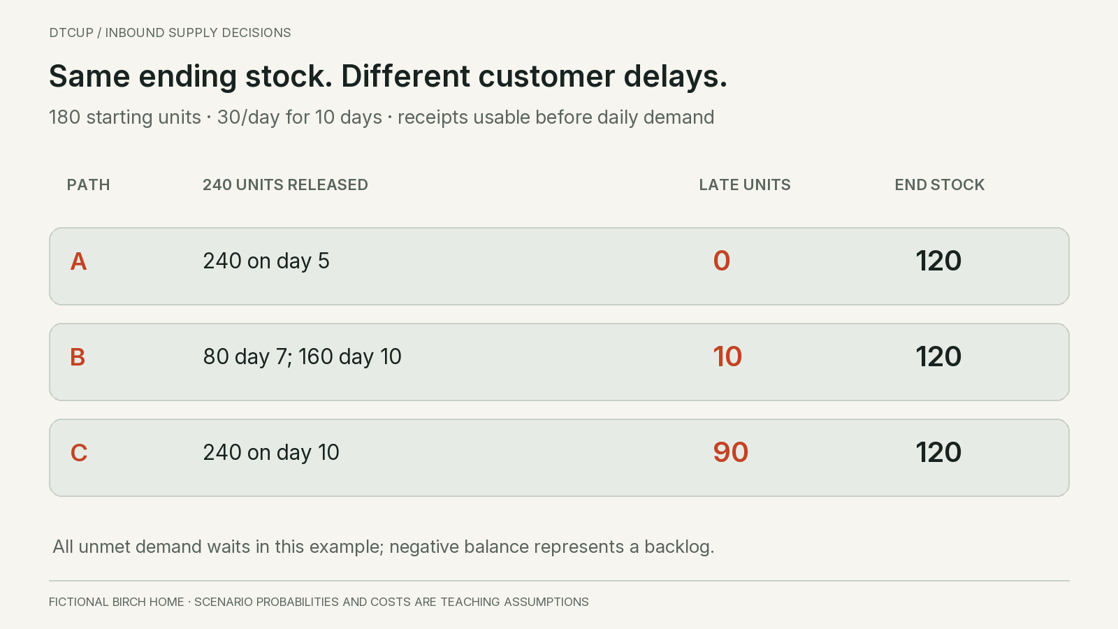
Scenario A releases all two hundred forty units before demand on day five. Birch consumes one hundred twenty units during the first four days, leaving sixty. The day-five receipt arrives before a shortage, so all three hundred units of horizon demand can be served on time and the ending balance is one hundred twenty.
Scenario B releases eighty units before demand on day seven and the remaining one hundred sixty before demand on day ten. The opening stock lasts through day six. After the first receipt and day-seven demand, fifty units remain. Day eight leaves twenty, and day nine creates a ten-unit deficit.
When the second receipt arrives on day ten, it can serve the ten waiting units and that day’s thirty units, leaving one hundred twenty. The same final stock as Scenario A conceals a different service outcome: ten units of demand waited for supply.
Scenario C releases all two hundred forty units before demand on day ten. After day six, there is no physical stock. Thirty units wait on day seven, another thirty on day eight and another thirty on day nine. The maximum backlog before the receipt is ninety units.
Day ten’s receipt serves that ninety-unit backlog and the current thirty units, again leaving one hundred twenty. Three plans with identical total demand, total supply and final balance produce zero, ten and ninety late units. A summary that shows only ending stock loses the decision that matters.
These paths are mutually exclusive descriptions of the same outstanding purchase order. They are not three separate orders to be added together. The spreadsheet or planning tool should make scenario identity explicit so that no report accidentally counts all of them as committed supply.
Partial receipts need usable quantities, not merely physical arrivals. If eighty units reach the dock on day seven but sixty remain on hold until day ten, the release path is twenty on day seven and the relevant later release. Calling the full eighty received does not make all eighty available for the service calculation.
Review each path with the people who own its assumptions. A plausible split requires confirmation that the supplier can separate the goods, transport can carry the partial shipment and the destination can receive and release it. A mathematically helpful split is not automatically an executable plan.
Do not turn expected receipts into a fictional shipment
Suppose the planning team assigns illustrative probabilities of fifty percent to Scenario A, thirty percent to B and twenty percent to C. These are assumptions for the calculation, not empirically estimated supplier probabilities. In practice, probabilities need evidence and calibration, or the plan should remain a set of unweighted scenarios.
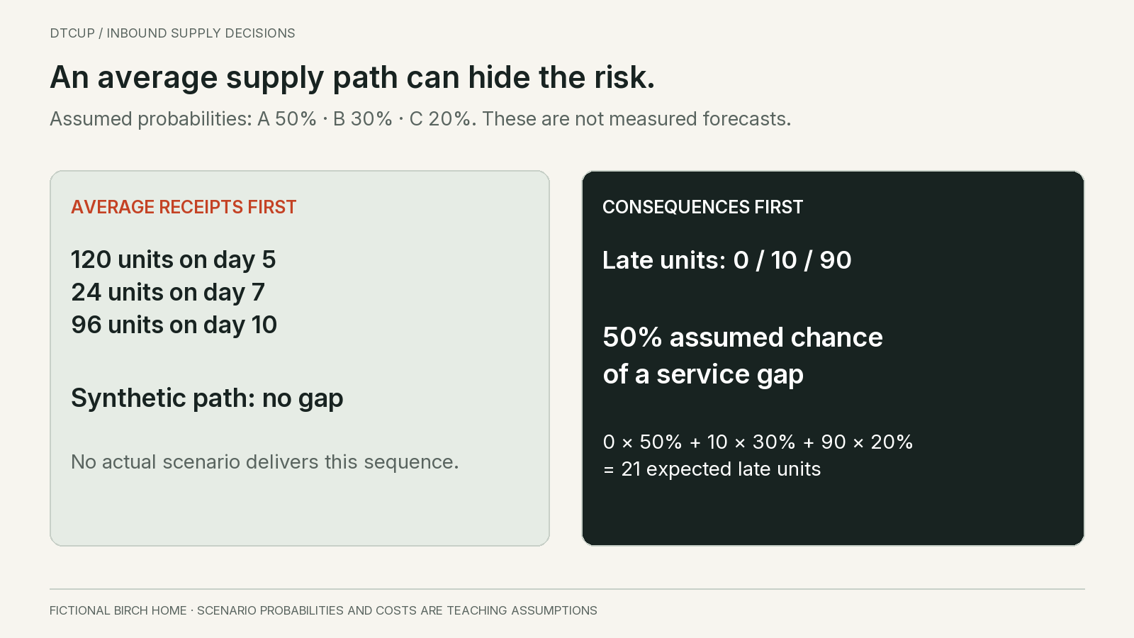
The probability-weighted receipt quantities are one hundred twenty units on day five, twenty-four on day seven and ninety-six on day ten. They sum to the same two hundred forty units. But no scenario actually delivers that sequence. It is an average across possible worlds.
If the planner runs the stock calculation on this averaged supply path, it shows no shortage. Sixty units remain after day four, the average day-five receipt raises the balance, and the later average quantities keep it positive. This can create a misleading conclusion that the plan is covered.
The actual scenario calculations say something else. Half of the assumed probability mass has a shortage: Scenario B contributes thirty percent and Scenario C twenty percent. Expected late units are twenty-one, calculated as zero times fifty percent, ten times thirty percent and ninety times twenty percent.
The reason is that shortage is not a linear property of average supply. An early receipt in one possible outcome cannot physically rescue a late receipt in a different outcome. Calculate the operational consequence inside each coherent scenario, then summarize those consequences if the probabilities are defensible.
An average ETA has a related limitation. It can describe a central tendency, but it does not tell the team how much supply is usable before a particular shortage date. A batch split across two dates cannot be represented fully by one date without losing important information.
Keep averages for the questions they can answer. Expected cost can help compare alternatives under explicit assumptions. It should not be displayed as a firm receipt schedule or used directly as a customer promise. Show the underlying scenarios and the range of service consequences beside it.
When the data is too thin for probabilities, use named cases such as confirmed path, plausible delay and severe disruption. The team can still choose a contingency based on consequences and decision deadlines. An honest scenario range is more useful than unsupported probabilities that make a dashboard appear scientific.
Update uncertainty when evidence changes, not when somebody feels optimistic
A confirmed milestone can remove some uncertainty and leave other uncertainty intact. Dispatch confirmation may settle whether the goods left the supplier. It does not necessarily settle customs timing, receiving capacity or inspection outcome.
Write what the new evidence changes. If production is complete but transport is unbooked, a production-delay scenario may become less relevant while transport-delay scenarios remain. Avoid replacing every uncertain date with one confident date just because a favorable update arrived.
Separate missing evidence from evidence of failure. A delayed tracking update does not by itself prove the shipment is lost. At the same time, silence should not be treated as confirmation that the original plan remains on track. The appropriate response is an exception with a named verification action.
Where historical data supports probabilistic planning, compare similar lanes, suppliers, product conditions and milestones. A factory-ready estimate and a warehouse-release estimate are not comparable errors. Preserve forecast snapshots made at consistent lead times so that the reliability analysis answers a meaningful question.
Check calibration over a suitable sample. If dates described as highly likely repeatedly miss, the labels need revision. A few successful receipts do not establish reliable tail probabilities, especially after a route, supplier or operating process changes.
Do not assume delays are independent when they share a cause. Two shipments on the same disrupted route, or several items waiting for the same component, can move together. Multiplying independent arrival probabilities can greatly understate a common disruption if independence is not credible.
Also avoid counting the same uncertainty twice. If the supplier’s stated date already includes a specific handling allowance, adding that allowance again changes the scenario. Keep real processing time, uncertainty protection and calendar rules visible enough to reconcile.
For the earlier stages and dependencies, use the purchase-order-to-sellable-stock lead-time guide. This scenario review starts where that map becomes a decision: which dated quantities can serve demand, what might change and which response is still possible.
Make inspection and partial release visible without weakening the checks
A shipment can physically arrive on time and still fail to support the plan. Documents may be missing, quantities may differ, or a quality process may require a hold. The planning record should show those conditions instead of blaming every service gap on transport.
Separate the quantity inspected from the quantity blocked. A sampling process can inspect a small subset while the entire lot remains unavailable pending a decision. The application configuration and quality procedure determine the scope. Do not assume that only the sample quantity is excluded from availability.
Similarly, avoid subtracting the same held units twice when two status systems describe the same restriction. An inspection hold and an unavailable inventory status might overlap. The sellable-stock calculation needs a reconciled set of physical units, not a sum of every negative-looking field.
If part of a lot can be released independently, identify the approved conditions and actual released quantity. A commercial deadline is not evidence that those conditions have been satisfied. Purchasing and marketing should not bypass the quality owner’s decision by relabeling goods as urgent.
For Birch’s split scenario, an eighty-unit release is useful because it almost bridges the demand until day ten. A twenty-unit release would have a different service effect. The planner should calculate the quantity actually available, then decide whether a separate contingency is still needed.
Receiving capacity is another constraint. A truck arriving late on a busy day may wait for a slot or miss the channel update cutoff. If this pattern is recurring, the solution may be a booked receiving appointment, better shipment information or a different release process rather than faster long-distance transport.
Keep the evidence of release attached to the planning event. The buyer should be able to distinguish an expected release from an actual release and see when the channel inventory was updated. These are operational controls that prevent a late physical handoff from becoming an inaccurate online promise.
Compare a contingency against the consequences it can actually change
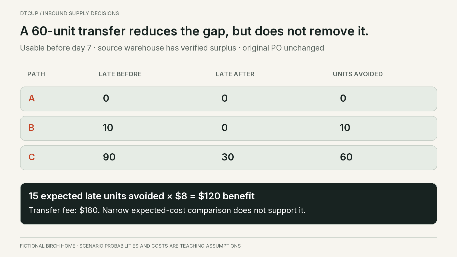
Suppose Birch can transfer sixty units from a second warehouse so they become usable before demand on day seven. For this example, that warehouse has verified surplus after protecting its own commitments and demand. The transfer costs one hundred eighty dollars and does not change the original purchase order’s receipt dates.
At the destination, Scenario A already had no shortage, so the transfer prevents no late units. Scenario B’s ten-unit gap disappears. Scenario C’s ninety-unit gap falls to thirty because the sixty additional units cover two of the three days before the original receipt.
Under the illustrative probabilities, expected late units fall from twenty-one to six: zero in A, zero in B and thirty times twenty percent in C. The transfer avoids fifteen expected late units. It does not eliminate the worst-case gap in the scenario set.
If the only avoidable consequence is eight dollars per late unit, the expected benefit is one hundred twenty dollars. That is less than the one hundred eighty dollar transfer cost. On that narrow expected-cost basis, paying for the transfer is not justified. The arithmetic is a decision aid, not a universal instruction to accept late service.
The decision can change if an important commitment has additional consequences, if the cost assumptions are wrong or if the business has a binding service requirement. Make those factors explicit. Do not quietly inflate the per-unit penalty until the calculation supports the preferred answer.
The transfer also leaves sixty more units at the destination after the horizon, assuming all demand waits and the original purchase order still arrives. The source warehouse loses those same units. Include the resulting location balance and any future replenishment adjustment rather than counting only the avoided gap.
The quoted transfer fee must cover the activities assumed in the option. Check picking, packing, transport, receiving and any extra handling separately if they are not included. The example assumes no additional source-location service loss; if that assumption fails, the transfer may move the shortage rather than reduce it. Evaluate both locations over the period affected by the move.
An option to decide later can have value, but its conditions must be real. If the transfer can be initiated on day six and still become usable before day-seven demand, new evidence may help avoid unnecessary cost. If it needs four days, waiting until day six destroys the option. Compare the action lead time with the decision deadline.
Evaluate expediting in the same way. Ask which quantity becomes usable earlier, whether that removes a specific gap and which downstream constraints remain. Paying for a faster leg that does not advance the usable date is not service protection; it is an expense with no modeled benefit.
Decide what unmet demand does before estimating commercial loss
The worked scenario carries every unserved unit forward until the receipt arrives. That makes late units visible and keeps the ending balance comparable. It is appropriate only for customers or demand that would actually wait under the stated conditions.
If all unmet demand is lost instead, Scenario C loses ninety units before day ten. The receipt then serves only day ten’s thirty units, leaving two hundred ten units physically on hand. The higher ending stock is not a better outcome; it reflects sales that did not occur.
Scenario B would lose ten units and finish with one hundred thirty, while A would still finish with one hundred twenty. A summary of ending inventory alone could therefore rank the most damaging delay as the best-stocked outcome. The customer-behavior assumption changes the interpretation.
Reality can contain a mixture of waiting, cancellation, substitution and later return. Use evidence where available and show a sensitivity range where it is not. Do not label all unmet demand as lost revenue or assume every late buyer returns automatically.
A substitution can move demand to another item and create a second shortage. If the business actively recommends an alternative, check that item’s available supply and margin. The response should not solve the original SKU’s problem by hiding the cost elsewhere.
For backorders, track the age and promise attached to waiting orders. Ninety units late for one day is different from ninety units late for several weeks. A unit count is only one service measure; duration, customer commitment and communication can change the consequence.
For lost sales, keep observed sales separate from estimated unconstrained demand. Otherwise a shortage reduces the history used by the next forecast, and the planner may order less precisely because the product was unavailable. The companion guide on demand hidden by stockouts explains that measurement problem.
Use the behavior model consistently when comparing contingencies. The eight-dollar late-unit cost above belongs to its stated backlog example. A lost-sale contribution calculation would need different assumptions and should not reuse that value without justification.
Coordinate the response across purchasing, fulfillment and customer promises
A revised receipt forecast should trigger a decision about both existing commitments and new demand. These are different audiences. Existing customers may need an update or an approved alternative; new visitors need an accurate availability statement before purchasing.
Do not publish the planner’s optimistic scenario as the default promise. Internal scenarios are tools for evaluating risk. A customer-facing date should pass the business’s approved evidence and service rules, with any conditions stated clearly.
For a promotion, compare the expected demand path with the usable receipt path. Delaying a campaign can reduce exposure, but it may have contractual, creative or commercial costs. Record the tradeoff rather than assuming demand can be switched off freely.
If the team reduces demand, update the scenario with a defensible new assumption. Merely lowering the forecast to match available stock does not change customer demand. A genuine action, such as moving a launch date or limiting an offer, should explain why the demand path changes.
Customer support should receive the same approved interpretation as the website team. A date in an internal logistics note should not be repeated as a guaranteed delivery date. Give staff the confirmed facts, unresolved conditions and permitted next steps.
AI assistants need the same boundary. A historical stock note or old arrival estimate should not override the current approved availability source. The assistant can explain the process and route the customer appropriately when a promise cannot be verified, rather than turning an internal ETA into certainty.
Set one owner for cross-team coordination. Purchasing can own supplier contact, the warehouse can own release and marketing can own campaign changes, but the overall exception needs a person who confirms that the resulting customer message matches the operational decision.
After a receipt becomes usable, verify that the selling channel reflects the actual released quantity. Closing the logistics issue before that last handoff can leave the website unavailable while stock sits ready, or available while the release is still incomplete.
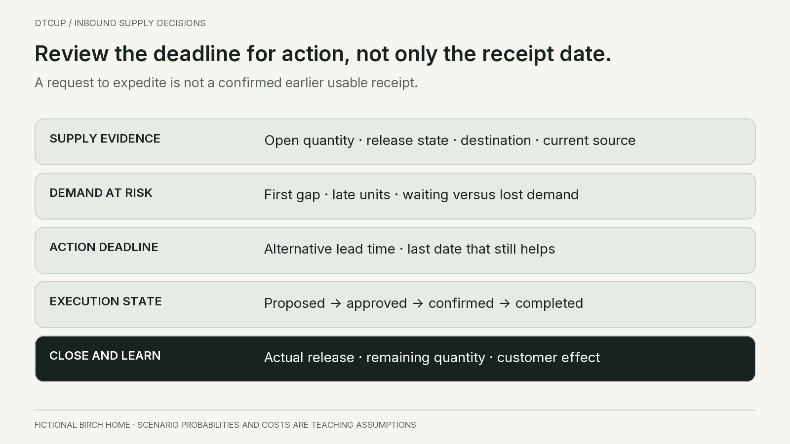
Run an exception review with a last useful action date
Start with the receipts that threaten a decision, not every open purchase order. A large order due next quarter may be less urgent than a small partial release needed before tomorrow’s customer cutoff. Rank by consequence and time to act.
For each exception, show the protected demand, current usable stock, relevant receipt paths and first gap date. Then show the available actions with their own lead times. This turns the meeting from a status recital into a choice.
Ask what evidence would change the decision before the deadline. A confirmed partial release may remove the need for a transfer. A missed booking may make an alternate route necessary. Assign the verification to a person and set a time that leaves room to execute the response.
Keep an action state that distinguishes proposed, approved, requested, confirmed and completed. A message asking for expedited freight is not a confirmed earlier receipt. The planning scenario should not count the benefit until its required evidence exists.
Record the original decision and assumptions before they are replaced by later information. Otherwise hindsight makes every outcome look obvious. The review should assess whether the action was reasonable with the information available, as well as whether it worked.
After the event, separate date error, quantity error and release delay. A supplier can deliver the promised quantity to the dock on time while an internal receiving backlog causes the service failure. Conversely, a warehouse can process promptly after a genuinely late delivery. Improvement depends on the actual cause.
Close the exception only after the remaining quantities, customer effects and system states reconcile. Partial completion may leave an outstanding balance or unresolved backorders. A single green delivered label should not hide those unfinished obligations.
Reconcile a partial receipt before updating the next plan
Take a separate receiving example using a two hundred forty unit purchase order. Eighty units physically arrive. Seventy-two pass the required checks and eight remain on hold. The supplier has not canceled the remaining one hundred sixty units. These facts create three distinct balances: seventy-two released, eight received but unavailable, and one hundred sixty still outstanding from the supplier.
The eight held units should not automatically be added to the supplier’s open quantity. They already arrived. If they later fail and the supplier agrees to replacements, record the replacement obligation explicitly under the agreed process. Otherwise the same eight units can appear both as held physical stock and as an undocumented future receipt.
Similarly, do not call the purchase order eighty units available just because eighty were counted at the dock. The available quantity is seventy-two under the example’s release rule. If some of those seventy-two are allocated to existing commitments, the uncommitted pool is smaller again.
A useful reconciliation identity is that the ordered quantity is accounted for by physically received quantity, documented cancellations and quantity still outstanding, subject to the system’s treatment of returns and amendments. Within the received quantity, released and held states must also reconcile without overlapping units. The exact fields vary by system, so agree on the identity before importing data.
Require the same care with units of measure. A supplier may report cartons while the website sells individual pieces. If each carton contains twelve pieces, eight cartons are ninety-six pieces, not eight. Keep the pack conversion effective for the actual item and shipment; a packaging change can invalidate a previously correct multiplier.
When the source is corrected, preserve the correction reason and timing. A count adjustment, an inspection release and a newly received delivery are different events. They should not all look like a new supplier shipment in the history used to assess receipt reliability.
Write the decision so another planner can challenge it
For Birch, the decision note begins with the protected task: serve thirty units of daily demand at the destination over ten days under the stated backlog assumption. It records one hundred eighty opening units and the three alternative paths for the same two hundred forty unit purchase order. That prevents the review from drifting into an unrelated monthly stock target.
The note then lists the evidence behind each path and clearly marks the illustrative probabilities as assumptions. In a real business, unsupported probabilities would be replaced by unweighted cases or estimates justified by relevant history. A precise percentage is not a substitute for explaining where the estimate came from.
Next, record the proposed sixty-unit transfer, its confirmed usable date and the source warehouse’s protected demand. State that it changes destination supply but not network supply, and that the original purchase order remains active. This makes the resulting extra destination stock visible rather than treating the transfer as a free temporary fix.
The commercial comparison follows: fifteen expected late units avoided under the assumed scenario weights, eight dollars of avoidable consequence per late unit, one hundred twenty dollars of expected benefit and one hundred eighty dollars of transfer cost. The narrow calculation does not support the transfer. Any decision to proceed anyway must name the additional service obligation or risk preference that justifies it.
Finally, list what would reopen the choice. A higher verified cost of delay, a lower transfer quote, a changed receipt path or a confirmed customer commitment could alter the decision. A vague instruction to monitor closely is less useful than identifying those triggers and the last time the transfer can still become usable before the gap.
Have a second person reproduce the quantity and cost calculations. They should be able to explain why every scenario ends with the same stock before the contingency but has a different service outcome. If they cannot, improve the record before relying on it to coordinate purchasing and customer communication.
After the actual receipt, add the observed path and customer effects without rewriting the original assumptions. A good outcome does not prove that a weak decision process was sound, and a bad outcome does not automatically prove that a reasonable probabilistic choice was wrong. Use the record to improve evidence, execution and future judgment separately.
Questions about uncertain inbound inventory
Can goods in transit be included in inventory planning?
Yes, as conditional dated supply with clear quantity, location and usability assumptions. They should not be confused with current sellable stock. The evidence needed for a customer promise may be stronger than the evidence used to explore an internal planning scenario.
Why not use a probability-weighted inbound quantity each day?
That average can create a receipt sequence that never occurs. Shortages depend on the path, so evaluate each coherent scenario first and then summarize the consequences. An early receipt in one outcome cannot physically compensate for a late receipt in another.
Should every delayed shipment be expedited?
No. Calculate which usable quantity arrives earlier, which service gap changes and what the action costs. Production, inspection or receiving constraints can prevent faster transport from improving the final usable date. Preserve residual risk and any effect on other locations.
Does a partial receipt prove the remaining order is reliable?
It proves something about the portion actually received and released. The remainder still needs its own current evidence and date. Reconcile the open quantity and avoid retaining the original full receipt alongside new partial lines.
What is the most useful first improvement?
Define usable stock and preserve original, current and actual receipt dates. Then take one threatened item through a daily demand-and-receipt scenario. That exercise usually reveals whether the immediate problem is missing evidence, duplicated supply, a release hold or an action taken too late.
A good inbound plan does not make uncertainty disappear. It makes the consequence of each plausible receipt path visible early enough to choose a response. That is the difference between knowing that stock is coming and knowing what the business can responsibly promise while it waits.
Sources
Still have a question?Ask the DTCUP Community ↗